30 Mar 17
Docs and Handoff — WA18
========================================================
Prediction Run — Pass II
* rebuilt tiling
– there was a bug in the tiling code that caused gaps, due to a floating point truncation; using %f format for the float, as input to the transform, was insufficient resolution and the tiles were slightly malformed
– after retiling Inglewood and Humboldt Arcata, re-run training and prediction
– take advantage of the change, and clip Humboldt to a water layer
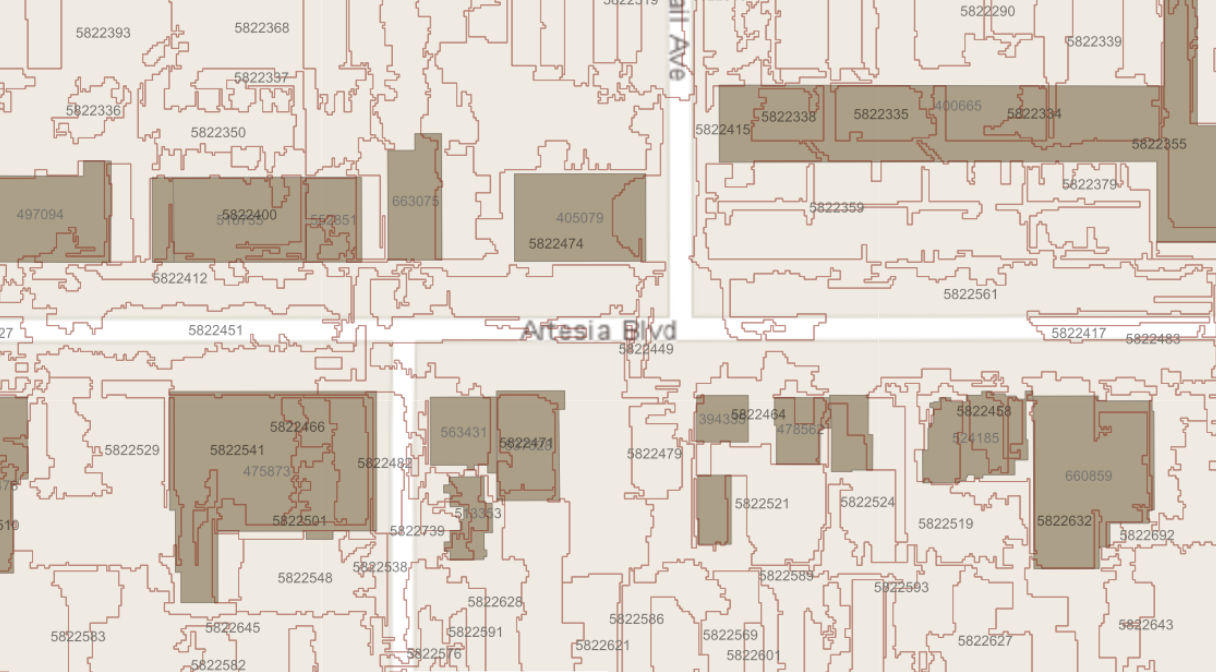
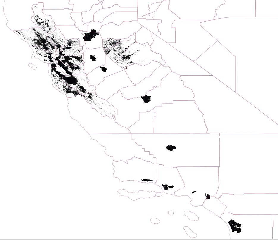
* Made a quick spatial join of Predicted set to Polys htarg2
– sent to garlynn for preliminary QC
– created a few QGis visualizations
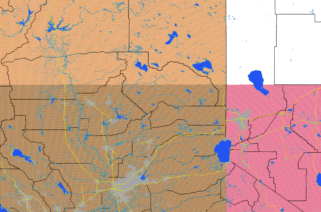
Humboldt Data
dist2road
Inglewood / Training
ctr_targ T/F; ctr_seg T/F; perc_overlap (0-1);
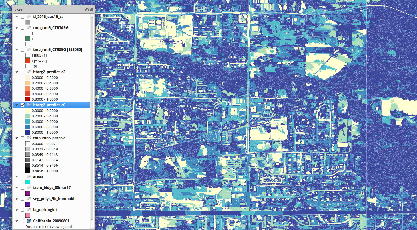
Humboldt / Prediction
coverage2 value (0-1);
MGRS Grid Reference
MGRS 10t 10s 11s start
buildings.buildings final
5563240 from all tables
5457201 removing duplicates
Google Earth Enterprise on Github
http://www.opengee.org/
Developer See is using SEGNET based ML
https://github.com/alexgkendall/caffe-segnet
https://github.com/developmentseed
https://www.developmentseed.org/projects/
24 Mar 17
Recognition Trials — WA18
========================================================
Machine Learning — Tuning the Training Process
The BIS2 segmentation engine has three paramaters. For this series of tests evaltest, the imagery zoom level is always “full image resolution” and only one NAIP DOQQ is segmented (a portion of Inglewood). Iterating through input parameters, segmentation is performed and the result polygons are saved. This is repeated many times, and for several ‘modes’ of the imagery. Valid imagery ‘mode’ starts with true color ‘tc’, false color ‘fc’ and infrared ‘ir’; new products such as a Sobel Filter result can be added. (20mar17 – first sobel-enhanced segmentation added)
In evaltest, 675 segmentation run combinations of (t,s,c,mode) at full resolution on NAIP 2016 imagery were executed and the results are stored as shapefiles on disk. A small python program (load-seg-data.py) loads the shapefiles into a spatial table.
The 675 tables test tables:
9 values for threshold (t) 10,20,30,40,50,60,70,80,90
5 values for shape (a) 0.1,0.3,0.5,0.7,0.9
5 values for compact (c) 0.1,0.3,0.5,0.7,0.9
3 values for mode ir,fc,tc
675 = 9 * 5 * 5 * 3
In the next step, statistics are calculated on the previous results (code in prep-relevance.py). These stats are saved in tables in the ma_buildings relevance schema. Tables have parameter values embedded in their names in a structured way (see below).
Completion of this step is to choose the best parameter set of a search objective. In this experiment, we are matching shape-to-shape. Python eval-stats.py generates SQL which contains a regular expression which filters the 675 tables of run result stats by encoded name, performs summary calculations on all rows in those tables (connected in the output by UNION ALL) and sorts all of that by a desired stats output column to discover outcomes in the test runs. Built-in Postgres math functions min() max() avg() stddev() are executed on three columns from each table, and counts of two more booleans. A SQL UNION ALL construct lists the chosen stats for all considered tables, one line per table, which then can be sorted in any way that is convenient to pick winners. Using this generalized format, statistics for any model run can quickly be compared. On the testing hardware, 450 tables of a few thousand rows each, are summarized and sorted for comparison in about 1.5 seconds.
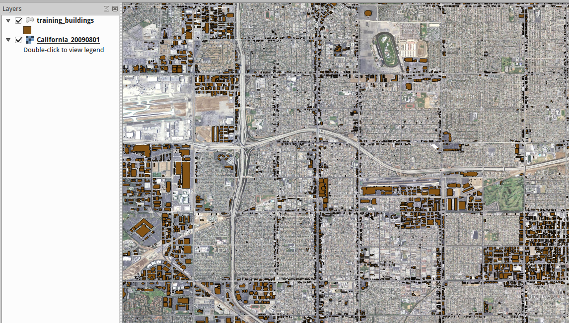
Visual display of segmentation in a Training Area of Inglewood, California.
-- Five Spatial Tests are Performed on Every Segment Intersecting a Training Building --

CREATE TABLE relevance.evaltest_evaltest1_MODE_T_S_C
(
  gid integer PRIMARY KEY,
  class integer,      -- 0 not considered;  2 commercial bldg
  pctoverlap double precision,
  coverage1 double precision,
  coverage2 double precision,
  centr_seg boolean,
  centr_trg boolean
)

-- Structure of a model run stats table  23mar17
--
ma_buildings=# select * from "5bandt1_test2_5b_50_03_03" limit 5;
  gid  | class |    pctoverlap     |     coverage1     |    coverage2     | centr_seg | centr_trg
-------+-------+-------------------+-------------------+------------------+-----------+-----------
 64311 |     2 | 0.547329611192823 | 0.970785850687081 | 35.9228431691447 | t         | f
 64559 |     2 | 0.137682284191657 | 0.836077333010945 | 0.54216208047878 | f         | f
 64107 |     2 |                 1 | 0.972281692288727 |   70.15447713594 | t         | f
 64698 |     2 | 0.728239585461471 | 0.924875366545267 | 17.6592649379458 | t         | f
 64721 |     2 | 0.923712040345278 | 0.943590470848252 | 30.8265007068801 | t         | f
(5 rows)


Relevance Query:
--    segmented poly (a)   < =  polys from a segmentation run w/ given params
--    target poly (b)      <=  training polys, what we are matching
--    raw areas (c)        <=  all known bldg polys in the area
--

        | insert into relevance.evaltest_evaltest1_fc_50_09_05
        |   select a.gid,
        |          1::integer,
        |          st_area(st_intersection(a.geom,c.geom))/st_area(a.geom),
        |          st_area(c.geom) - st_area(st_intersection(a.geom,c.geom))
        |            + abs(st_area(a.geom) - st_area(c.geom)),
        |          (st_area(c.geom) - st_area(st_intersection(a.geom,c.geom)))
        |            / st_area(a.geom),
        |          st_intersects(st_centroid(a.geom), c.geom),
        |          st_intersects(st_centroid(c.geom), a.geom)
        |     from seg_polys a
        |          join raw.areas c on st_intersects(a.geom, c.geom)
        |           left outer join
                       relevance.evaltest_evaltest1_fc_50_09_05 b on a.gid=b.gid
        |    where b.class is null  and
               jobid='evaltest'  and  project='evaltest1'  and
               mode='fc'  and  t=50.000000  and  s=9.000000  and  c=5.000000
                 on conflict do nothing
Relevance Tests
pctoverlap => the area of the intersection between the target training poly and a segmented poly, divided by the total area of the segmented poly; meaning, the percentage of the segmented poly that is intersecting the target, converges to 1.0 on a segmented poly that is entirely intersecting the target
cov1 => the area of a building that is not covered by the intersection with the segmentation poly plus the absolute value of the difference between the segmented poly and the building poly; meaning, a measure of non-fit; converges to zero on a perfect fit (actually, we changed this again, see code)
cov2 => the area of the segmented poly outside of the intersection with the target, divided by the area of the segmented poly; meaning, the proportion of the poly that is not part of the target fit; converges to 0 on a perfect fit
eval-stats.py -m tc -f cov1 -o avg -g

  search all result tables in schema 'relevance' for test run summary tables matching
imagery mode 'tc' True Color with any parameters; from those tables,
calc min() max() avg() and stddev() on all measures, but emit only the totals for the chosen column 'cov1',
one line per table; sort those results on column 'average' with the default sort order
of smallest first. In this example, segmentation parameter 20-07-07 gave the lowest
average value of cov1 for all test runs, with 20-07-03 closely following.

  table                         class count minimum   maximum   average   stddev  centr_seg centr_trg
----------------------------------------------------------------------------------------------------------
evaltest_evaltest1_tc_20_07_07   1   7237   0.000324  0.801199  0.052418  0.083101   3420   1414
evaltest_evaltest1_tc_20_07_03   1   6694   0.000476  0.800666  0.052979  0.083563   3158   1336
evaltest_evaltest1_tc_30_05_09   1   5404   0.000354  0.800875  0.053037  0.084356   2406   1232
evaltest_evaltest1_tc_30_03_09   1   6731   0.000324  0.800875  0.053139  0.082947   3202   1362
evaltest_evaltest1_tc_40_01_07   1   5310   0.000468  0.899413  0.053150  0.084180   2394   1223
evaltest_evaltest1_tc_30_05_03   1   5252   0.000320  0.801222  0.053332  0.082887   2362   1209
evaltest_evaltest1_tc_30_01_01   1   8033   0.000331  0.801431  0.053378  0.082763   3932   1425
evaltest_evaltest1_tc_30_01_05   1   8069   0.000331  0.800875  0.053403  0.081330   3936   1451
evaltest_evaltest1_tc_30_01_07   1   8212   0.000394  0.801083  0.053454  0.082504   4053   1459
evaltest_evaltest1_tc_20_05_03   1   9560   0.000320  0.801222  0.053536  0.081324   4769   1530
evaltest_evaltest1_tc_30_05_05   1   5379   0.000531  0.800875  0.053862  0.083052   2403   1210
evaltest_evaltest1_tc_20_05_05   1   9607   0.000476  0.801410  0.053940  0.083886   4795   1542
evaltest_evaltest1_tc_30_03_05   1   6658   0.000320  0.800875  0.054063  0.083892   3125   1324
-- Classified Segments with a Given Band and Segmentation --

ma_buildings=# select class, count(*) from evaltest_evaltest1_ir_50_01_03 group by class;
 class | count
-------+-------
     1 |  4708
     2 |   324
(2 rows)
Topics in Training Target Selection
Process Steps
- Generate 2000x2000 pixel tiles in the Training Area and the Search Area
done -- 80 in Inglewood and 130 in Humboldt - Segment those tiles done -- chose 50_03_03
- Load that segment data into the database done -- table sd_data.seg_polys_5b
- Feed the segment data to ML tools (either train or predict)
predict-segments.py and train-segments.py - Write the ML results back to the database.
Building Size
Very small buildings are more likely to be confused with other kinds of visible features, therefore remove training target buildings smaller than 90 m-sq
Next, what is a reasonable cutoff for buildings between 90 m-sq and MAX_SIZE
This is a stats distribution question.. We know the buildings of interest (commercial) look very much like other buildings. What is are identifying characteristics of commercial buildings that will help distinguish them from all buildings? Looking at distributions of features on all buildings is some curve, and the features of buildings we are looking for in the training set is a different curve.. Non-commercial buildings will have more occurrences in the low sq-m sizes, making false matches to commercial buildings more likely.
Let's start simple.
A quick look at the full training set shows that roughly 90,000 of the 250,000 bldgs are less than 150 m-sq, which means that 160,000 or 64% are >= 150 m-sq . My first reaction is ... look for >= 150 m-sq
--
20Mar17 Next Up
Segmentation is a general-purpose topic in imaging right now, so inevitably there will be other toolkits and advanced researchers that use it.. Some parts of the setup now would have to be generalized to handle other segmentation engines, but that is "out of scope" for this pass. For example, masking, poly splitting and poly merging, are well know in image segmentation. We have many options to explore, but must prioritize as we make the best use of the BIS2 tool we started with..
We have successfully added a fifth band to the raster layer 'mode'='sobel'.
Using this five-band input, combined with segmentation trials, definitely
improves the result. The toolchain did not have to change other than add the new layer.
Documenting the details of this is better left at the code level.
revised relevance query:
insert into relevance."inglewood_run1_5b_50_03_03"
     1::integer,
     -- pctoverlap
        st_area(st_intersection(a.geom,c.geom))/st_area(a.geom),
     -- coverage1
        (st_area(c.geom) + st_area(a.geom) -
         2.0*st_area(st_intersection(a.geom,c.geom))) /
          (st_area(c.geom) + st_area(a.geom)),
     -- coverage2
        (st_area(c.geom) - st_area(st_intersection(a.geom,c.geom)))
          / st_area(a.geom),
     -- centr_seg
        st_intersects(st_centroid(a.geom), c.geom),
     -- centr_trg
        st_intersects(st_centroid(c.geom), a.geom)
   from seg_polys_5b a                                 -- (3) segment polygons
    join la14.lariac4_buildings_2014 c on st_intersects(a.geom, c.geom) -- (4) building polygons
      left outer join relevance."inglewood_run1_5b_50_03_03" b on a.gid=b.gid
       where b.class is null  and  jobid='inglewood'  and  project='run1'  and
         mode='5b'  and  t=50.000000  and  s=3.000000  and  c=3

 -- previous
 select a.gid,
    1::integer,
    -- pctoverlap
    st_area(st_intersection(a.geom,c.geom))/st_area(a.geom),
    -- coverage1
    (st_area(c.geom) + st_area(a.geom) -
      2.0*st_area(st_intersection(a.geom,c.geom))) /
        (st_area(c.geom) + st_area(a.geom)),
    -- coverage2
    (st_area(c.geom) - st_area(st_intersection(a.geom,c.geom)))
      / st_area(a.geom),
    -- centr_seg
      st_intersects(st_centroid(a.geom), c.geom),
    -- centr_trg
      st_intersects(st_centroid(c.geom), a.geom)
 from seg_polys_5b a
        join raw.areas c on st_intersects(a.geom, c.geom)
          left outer join relevance."5bandt1_test2_5b_50_03_04" b on a.gid=b.gid
 where
    b.class is null  and  jobid='5bandt1'  and  project='test2'  and  mode='5b'  and
    t=50.000000  and  s=3.000000  and  c=4.000000
      on conflict do nothing

--
train-segments.py
  from sklearn.neighbors import KNeighborsClassifier
  from sklearn.ensemble  import GradientBoostingClassifier


--
ma_buildings=# \d inglewood_run1_5b_50_03_03
Table "relevance.inglewood_run1_5b_50_03_03"
   Column   |       Type       | Modifiers
------------+------------------+-----------
 gid        | integer          | not null
 class      | integer          |
 pctoverlap | double precision |
 coverage1  | double precision |
 coverage2  | double precision |
 centr_seg  | boolean          |
 centr_trg  | boolean          |
Indexes:
    "inglewood_run1_5b_50_03_03_pkey" PRIMARY KEY, btree (gid)

50-03-03
We selected this parameter set to use for the test area.. It is good at selecting a lot of area from a large, single roof. Complex roofs that have colored parts, using the training tests we have, do not get joined using these settings.
dist2road
This measure seems important, yet it is a substantial cost to calculate, at least the way we are doing it now.
 5415961.887 ms  statement:
   update sd_data.seg_polys_5b a
    set dist2road=(select st_distance(a.geom, b.geom) from roads b
        order by b.geom < ->a.geom limit 1)
     where dist2road is null and a.gid between 400001 and 500001
Completed Prediction Run
NAIP 2016 60cm segmented; predicted and classified based on Inglewood_5b model, sklearn Gradient Boost Tree (GBT).
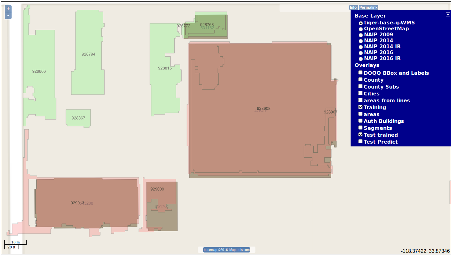
Inglewood_5b training polygons, alongside classified segmented polygons
## Complete Machine-Learning Pipeline pass
##  23March17 -dbb

# tile the cousub for inglewood
./tile-area.py -o inglewood -f 0603791400 -s 2000 -m 5b

# segment all the tiles in the inglewood directory
./segment-dir.py -m 5b -t 50 -s 0.3 -c 0.3 inglewood/

# load all the segment polygons into the database, compute dist2road
# with jobid=inglewood, project=run1
# segments go into sd_data.seg_polys_5b
./load-seg-data.py -p run1 -m 5b inglewood inglewood/

# compare the segment polygons to the training polygons
# filtering any training polygons less than 150 sq-m in area
# save the results in relevance.inglewood_run1_5b_50_03_03
./prep-relevance.py -b inglewood_run1_5b_50_03_03 -j inglewood -p run1
-m 5b -t 50 -s 0.3 -c 0.3 -z 150

# Using scikit learn and Gradient Boost Tree ML module
# train it using the segments in the database
# and save the trained object in inglewood_run1_5b_50_03_03-r0.5.pkl.gz
./train-segments.py -j inglewood -p run1 -m 5b -r 0.5 -b
inglewood_run1_5b_50_03_03 inglewood_run1_5b_50_03_03-r0.5.pkl.gz

# tile an area for Humboldt based on a bounding box
# and place the tiles in directory humboldt
./tile-area.py -o humboldt -b -124.17664,40.85411,-124.05923,41.00326 -s
2000 -m 5b

# segment all the tiles in the humboldt directory
./segment-dir.py -m 5b -t 50 -s 0.3 -c 0.3 humboldt/

# load all the segment polygons into the database, compute dist2road
# with jobid=humboldt, project=target
# segments go into sd_data.seg_polys_5b
./load-seg-data.py -p target -m 5b humboldt humboldt/

# run the trained classifier inglewood_run1_5b_50_03_03-r0.5.pkl.gz
# against the humboldt segments and save the results to
# predict.humboldt_target_5b_50_03_03_r005
./predict-segments.py -b humboldt_target_5b_50_03_03_r005 -j humboldt -p
target -m 5b inglewood_run1_5b_50_03_03-r0.5.pkl.gz
Visualized output per parameter set:
http://ct.light42.com//osmb/?zoom=19&lat=33.87306&lon=-118.37408&layers=B000000FFFFFTFFT&seg=evaltest_evaltest1_tc_70_03_07
http://ct.light42.com/osmb/?zoom=19&lat=33.87306&lon=-118.37408&layers=B000000FFFFFTFFT&seg=evaltest_evaltest1_tc_70_03_05
Other Topics
ECN OSM Import
https://github.com/darkblue-b/ECN_osm_import/blob/master/load-osm-buildings.cpp
BIDS
https://bids.berkeley.edu/news/searchable-datasets-python-images-across-domains-experiments-algorithms-and-learning
OBIA
http://wiki.landscapetoolbox.org/doku.php/remote_sensing_methods:object-based_classification
https://www.ioer.de/segmentation-evaluation/results.html
https://www.ioer.de/segmentation-evaluation/news.html
OSM
https://wiki.openstreetmap.org/wiki/United_States_admin_level#cite_ref-35
Jochen Topf reports that the multi-polygon fixing effort is going well and provides an issue thread to track the evolution.
https://blog.jochentopf.com/2017-03-09-multipolygon-fixing-effort.html
https://github.com/osmlab/fixing-polygons-in-osm/issues/15
-
On Mar 22, 2017 9:59 AM, "Brad Neuhauser"
> I think this is it?
> http://wiki.openstreetmap.org/wiki/Available_Building_Footprints
>
> On Wed, Mar 22, 2017 at 11:54 AM, Rihards
>
>> On 2017.03.22. 18:37, Clifford Snow wrote:
>> > I am happy to announce that Microsoft has made available approximately
>> > 9.8 million building footprints including building heights in key
>> > metropolitan areas. These footprints are licensed ODbL to allow
>> > importing into OSM. These footprints where manually created using high
>> > resolution imagery. The data contains no funny field names such as
>> > tiger:cfcc or gnis:featureid or fcode=46003, just building height.
>> >
>> >
>> > Please remember to follow the import guidelines.
>> >
>> > The wiki [1] has more information on these footprints as well as links
>> > to download.
>>
>> the link seems to be a copypaste mistake 🙂
>>
>> > [1] http://www.openstreetmap.org/user/dieterdreist/diary/40727
>> >
>> > Enjoy,
>> > Clifford Snow
>> >
>> >
>> > --
>> > @osm_seattle
>> > osm_seattle.snowandsnow.us
>> > OpenStreetMap: Maps with a human touch
>> >
>> >
NGA
https://apps.nga.mil/Home
Development Seed
https://developmentseed.org/blog/2017/01/30/machine-learning-learnings/
17 Mar 17
Recognition Trials -- WA18
========================================================
“object-based approaches to segmentation ... are becoming increasingly important as
the spatial resolution of images gets smaller relative to the size of the objects of interest. ”Andy Lyons, PhD
University of California, Division of Agriculture and Natural Resources
Informatics in GIS -LINK-
Topics for Detecting Buildings in Aerial Imagery:
- Object-based Image Analysis versus Pixel-based Image Analysis redux
- Change-detection using multi-temporal imagery
- Inherent Difficulty of Identifying Buildings in Imagery, even for a human
- LIDAR can increase detection dramatically, but is difficult to scale
Topics in Segmentation
- Object-based Image Analysis relies on Segmentation
- removing roads before segmentation
- removing vegetation before segmentation using IR layer
- using height information and shadow-detection
Measuring Success
- positive match rate to ground truth
- miss rate to ground truth
- false positives
- false negatives
Although many image segmentation methods have been developed,
there is a strong need for new and more sophisticated segmentation
methods to produce more accurate segmentation results for urban object
identification on a fine scale (Li et al., 2011).
Segmentation can be especially problematic in areas with low contrast
or where different appearance does not imply different meaning. In this
case the outcomes are represented as wrongly delineated image objects
(Kanjir et al., 2010).excerpted from:
URBAN OBJECT EXTRACTION FROM DIGITAL SURFACE MODEL AND DIGITAL AERIAL IMAGES Grigillo, Kanjir -LINK-
research with examples of Object-based Image Analysis (OBIA):
An object-oriented approach to urban land cover change detection. Doxani, G.; Siachalou, S.; Tsakiri-Strati, M.; Int. Arch. Photogramm. Remote Sens. Spat. Inf. Sci 2008, 37, 1655–1660. [Google Scholar]
Monitoring urban changes based on scale-space filtering and object-oriented classification. Doxani, G.; Karantzalos, K.; Strati, M.T.; Int. J. Appl. Earth Obs. Geoinf 2012, 15, 38–48. [Google Scholar]
Building Change Detection from Historical Aerial Photographs
Using Dense Image Matching and Object-Based Image Analysis -LINK-
Nebiker S., Lack N., Deuber M.; Institute of Geomatics Engineering, FHNW University of Applied Sciences and Arts Northwestern Switzerland, Gründenstrasse 40, 4132 Muttenz, CH
more research -LINK-
A Few Definitions:
GSD -- ground sampling distance; real distance between pixel centers in imagery
DSM -- Digital Surface Model; similar to Digital Elevation Model
eDSM -- extracted Digital Surface Model; post-process result, varying definitions
nDSM -- normalized Digital Surface Model; varying definitions
FBM -- Feature-based mapping; store only features, not empty spaces
SGM -- Semi-global matching; computationally efficient pixel analysis
morphological filtering -- computationally efficient edge methods
automated shadow detection -- in OBIA
Hough Transform -LINK-
Representative Public Test Process:
ISPRS Commission III, WG III/4
ISPRS Test Project on Urban Classification and 3D Building Reconstruction
![]() "... you dont want to be fooling with a lot of parameters.. you want paramater-free functions whenever you can.. thats one thing I think is exciting about neural networks (and the like), is that you just throw some images in there, and out come some magic answers. I think we will be seeing more of that."
"... you dont want to be fooling with a lot of parameters.. you want paramater-free functions whenever you can.. thats one thing I think is exciting about neural networks (and the like), is that you just throw some images in there, and out come some magic answers. I think we will be seeing more of that."
scikit-image: Image Analysis in Python / Intermediate
SciPy 2016 Tutorial * Stefan van der Walt
Machine Learning Pipeline Components
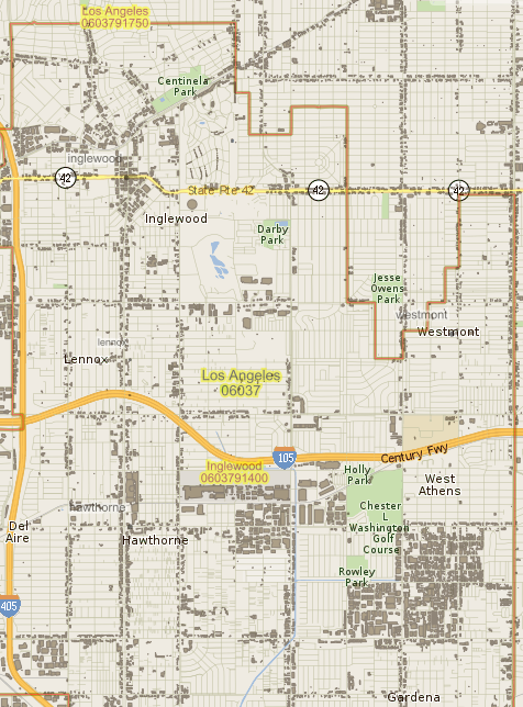
Training buildings available in Inglewood, Calif.
Known-good Building Polygons all have the following attributes available:
ma_buildings=# \d train_bldgs_08mar17
                 Table "sd_data.train_bldgs_08mar17"
          Column           |            Type             | Modifiers
---------------------------+-----------------------------+-----------
 gid                       | integer                     | not null
 building_type_id          | integer                     |
 building_type_name        | text                        |
 situscity                 | text                        |
 shp_area_m                | integer                     |
 geom                      | geometry(MultiPolygon,4326) |
 naip_meta_1               | integer                     |
 naip_meta_2               | text                        |
 urban_ldc                 | integer                     |
 compact_ldc               | integer                     |
 standard_ldc              | integer                     |
 intersection_density_sqmi | double precision            |
 acres_grid_gf             | double precision            |
 acres_grid_con            | double precision            |
 use_du_dens               | double precision            |
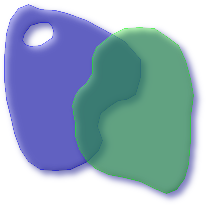
Theory of Determination of Relevance -- Clinton_Scarborough_2010_PERS
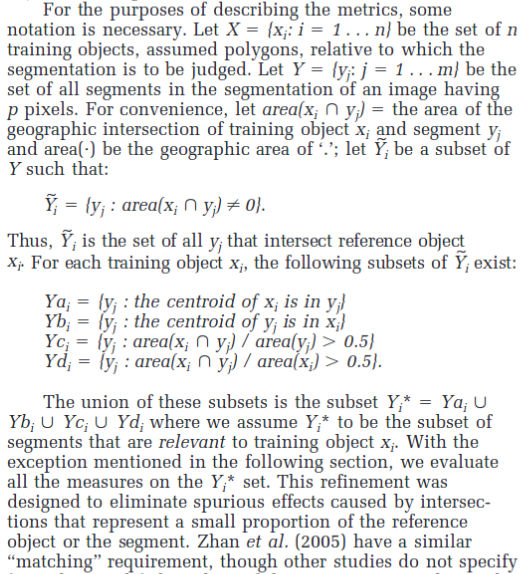
from Accuracy Assessment Measures for Object-based Image Segmentation Goodness: Clinton, et al
Pipeline Tools to date:
prep-relevance.py  >options<
  create a table associated with subset of seg_polys and assign
  to a class based on mutual percent overlap with a truth polygon

  options:
    -h|--help
    -i|--info  - report available jobid, project, t, s, c parameters and exit
    -b|--table tablename - table to create with relevance and class code (required)
    -j|--jobid name          -+
    -p|--project name         |
    -m|--mode ir|tc|fc|4b     |- filters for selecting specific records
    -t|--threshold n.n        |
    -s|--shape n.n            |
    -c|--compact n.n         -+
    -v|--verbose
Segmentation Trials -LINEUP-
train-segments.py
Usage: train-segments.py >options< trained-object.pkl.gz
    -i|--info  - report available jobid, project, t, s, c parameters
    -b|--table tablename - table with relevance and class code
    -j|--jobid name    -+
    -p|--project name   |
    -t|--threshold n.n  |- filter dataset to be extracted
    -s|--shape n.n      |
    -c|--compact n.n   -+
    -r|--relevance n.n - min relevance value to be part of class, default: 0.5
    -v|--verbose
    -x|--test - Use 50% of data to train and 50% to predict and report
    -a|--algorithm - KNN - KNearestNeighbors|
                     GBT - Gradient Boost Tree, default: GBT

   conn = psycopg2.connect("dbname=ma_buildings")

predict-segments >options< trained-object.pkl.gz
    -i|--info  - report available jobid, project, t, s, c parameters
    -b|--table tablename - table to create with relevance and class code
    -j|--jobid name    -+
    -p|--project name   |
    -t|--threshold n.n  |- filter dataset to be extracted
    -s|--shape n.n      |
    -c|--compact n.n   -+
    -x|--test - do the prediction but don't write to the database


eval-stats.py
    scan intermediate relevance tables and compute descriptive statistics

eval-segmentation.py
  evaluate multiple t, s, c parameters of the segmentation process
  and try to pick the that gives up the best results

  for a given training set:
    * take 40% of the polygons and use them for training
    * take 40% of the polygons and use them for evaluation
    * save 20% of the polygons as a hold back set for final evaluation

  there are currently two proceses planned to do this:
  1. a short path:
     compute the relevance for all the polygons
     and try to increase the average mutual coverage
     and decrease the stddev on the average mutual coverage
     take the best 2-3 sets of parameters and run them through 2.

  2. a long path: (NOT IMPLEMENTED YET)
     compute the relevance for all the polygons
     create a trained classifier using the training polygons
     run the test polygons through the trained classifier
     evaluate the goodness of the fit

  In either case, save the parameters that gave the best fit.

  Relevance tables will be generated based on >jobid< >project< t s c

-------------------------------------------------------
load-seg-data.py [-c] jobid dir
  -c    - optionally drop and tables
  jobid - string to uniquely identify this data
  dir   - segmentizer output directory to walk and load

For a given input file like project/tcase/test-fc.vrt
the segmentizer generates files in path project/tcase/:

test-fc.vrt_30_05_03.tif
test-fc.vrt_30_05_03.tif_line.tif
test-fc.vrt_30_05_03.tif_rgb.tif
test-fc.vrt_30_05_03.tif_stats.csv
test-fc.vrt_30_05_03.tif.shp

We can generate files given this matrix:

  mode |  t  |  S  |  c  |  z  |
  ------------------------------
   fc  | 30  | 05  | 03  | 19  |
   ir  | 50  | ... | 07  | ... |
   tc  | ... | ... | ... | ... |
  ------------------------------

We can generate any number of values for t, s, c, and z.
Segmented results are stored in table seg_polys,

create table sd_data.seg_polys (
  gid serial not null primary key,
  project text,               -- from file path
  tcase text,                 -- from file path
  ...

--
segment-dir options dir
    Call the segmentation engine for each file in a directory, with the given settings
    Produce an HTML overview for human interpretation of results

      [-t|--threshold T]   - T1[,T2,...] thresholds, default: 60
      [-s|--shape S]       - S1[,S2,...] shape rate, default: 0.9
      [-c|--compact C]     - C1[,C2,...] compact/smoothness, default: 0.5
      [-v]                 - be verbose
      [--nostats]          - don't generate stats.csv file
      [--nolineup]         - don't generate the lineup image


--
The following database table enables reference of any dataset from a mapfile:

create table sd_data.seg_tileindex (
  gid serial not null primary key,
  project text,               -- from file path
  tcase text,                 -- from file path
  ...
Other Imaging Filters Dept.
A Sobel Filter from sckit-image may be worth adding to the chain
The filter detects edges well (though they are not squared and various weights).
A target area could be passed through the filter and added as a segmentation clue.
08 Mar 17
Recognition Trials -- WA18
========================================================
Project Big Picture
"tripartite solution" -- Authoritative Sources of 2D building footprints, with varying attributes (dbname=auth_buildings), updates and ingestion are semi-manual; Openstreet Buildings with minimal attributes (dbname=osm_buildings), updates are automated; Machine-Learning generated building locations (dbname=ma_buildings), updates are machine-generated with supplementary attributes.
ML Theory
Unsupervised Classification with pixel-based analysis (see below)
Supervised Classification with Object-based analysis (what we are using, newer)
Project Details
Database ma_buildings schemas now include: building_types, a classification system for buildings in all use_codes; US Census TIGER, road network, block groups, county subportions; Grid 150m Los Angeles County, vast, high-resolution landuse and urban metrics data; LARIAC4 Buildings 2014, every building in LA from SCAG; sd_data training_buildings, a table-driven source of ML training targets (see below), picked from 249,927 classified geometry records of commercial and MF5+ buildings in LA County.
Building a Training Set: filter a set of 2D building polygons of interest from LA County (table=sd_data.train_bldgs); run a segmentation on remote sensing data layers NAIP 2016, store the results (table=seg_polys).
Recognition: Segment a target search area using remote sensing layers NAIP 2016; use ML engine and training product to recognize likely matches; characterize the results.
Documentation & Handoff
discussion
* Training Set, continued:
- Garlynn's crosswalk JOIN table gives a LOT of category information on the buildings themselves. In effect, takes 300,000 or so non-residential buildings and puts a very fine grain classification on them.
"Each and Every Building in LA, provided by the County"
ma_buildings  la14.lariac_buildings_2014
----------------------------------------
code, bld_id, height, elev,
lariac_buildings_2014_area, source, date_, ain, shape_leng, status, old_bld_id,
 ...

"Building Categorization from Vision_California release"
building_types
--------------------------------------------------------
  building_type_category text,
  building_type_id integer NOT NULL,
  building_type_name text,
  building_height_floors integer,
  total_far integer
  ...

UseCode_2_crosswalk_UF_Building_Types2.csv
-------------------------------------------
usecode_2,usetype,usedescription,bt_id,mf5_plus_flag,include_flag
10,Commercial,Commercial,41,,1
11,Commercial,Stores,41,,1
12,Commercial,Store Combination,39,,1
13,Commercial,Department Stores,39,,1
14,Commercial,Supermarkets,41,,1
15,Commercial,"Shopping Centers (Neighborhood, community)",41,,
16,Commercial,Shopping Centers (Regional),39,,1
17,Commercial,Office Buildings,32,,1
18,Commercial,Hotel & Motels,38,,1
19,Commercial,Professional Buildings,32,,1
....
First attempt at a JOIN with a VIEW.. did not work for QGis and had permissions problems within the database. Second attempt simply defines a TABLE in the sd_data schema. Success !
First pass at a finely categorized non-residential building set in LA County as ML Training Set candidates.
Misc URLs
http://ct.light42.com/osmb/work/lineup.html
http://ct.light42.com/osmb/la14-50-60-09-05/lineup.html
http://ct.light42.com/osmb/la14-50-60-09-01_05_07/lineup.html
.. and, Machine Learning problematic data
http://ct.light42.com/osmb/?zoom=18&lat=33.92182&lon=-118.35224&layers=000000BFFTFFTFF
Characterize Training Set Buildings
- residential multifamily five units and up - are included
- how many buildings ? what sizes ? no filter on "small bldgs" yet
Attributes and Sources For Training Set (gw):
- Should record imagery attributes (direction of sun angle, year, etc). This will come from the NAIP metadata. WHY: It obviously matters from which direction the sun is shining, as shadows will be found on the opposite sides of objects from the sun. Time of year will tell about the presence or absence of leaves on deciduous vegetation. The year allows for time-series comparisons between different vintages of the same dataset.
- City (name) — this can come from a number of sources, including the LARIAC buildings shapes themselves (SitusCity). WHY: Different cities may have different attributes, citywide, in a meaningful manner.
- The area of the polygon, from LARIAC buildings training set (Shape_Area). WHY: We want to be able to filter by this attribute for only large buildings.
- urban_ldc from the UF base grid. WHY: These are super-urban areas, more than 150 walkable intersections/sqmi, most buildings here are skyscrapers.
- compact_ldc from the UF base grid. WHY: These are compact development types, more than 150 walkable intersections/sqmi, with a walkable street grid.
- standard_ldc from the UF base grid. WHY: These are suburban development types, less than 150 walkable intersections/sqmi,
- intersection_density_sqmi from the UF base grid. WHY: Intersection density is a critical variable in urbanism. It could be that the machine finds a strong correlation between it and other things. Let’s find out.
- acres_grid_gf from the UF base grid. WHY: Greenfield acres tell us how many non-urbanized acres are within the grid. If this is above some threshold, say 85% of the grid cell, we can probably skip that grid cell for ML analysis.
- acres_grid_con from the UF base grid. WHY: Constrained acres also tell us how many non-urbanized acres are within the grid. If this is above some threshold, say 85% of the grid cell, we can probably skip that grid cell for ML analysis.
- use_du_dens from the UF base grid. WHY: We may be able to do something clever, like filter out the residential records from the buildings dataset by only those grid cells from the UF base load with a DU use density above some threshold (I’m thinking 10-20 or so), which should get rid of some of the noise in the data.
- Building Size -- Filter all records by our threshold size: 2,000? 10,000? ...of 2D footprint. Maybe don’t try this during the first pass? Keep it in your back pocket for later? Not sure.
Server Layout
 /var/local/osmb_ab/
    bin        # all automation, plus small utils
        add-auth-building-layer  do-backup            json-to-postgres    osm_building_stats
        create-auth-buildings    extract-image.py     load-osm-buildings  reload-osm-buildings
        createdb-dee1            fetch-osm-ca-latest  load-roads          wget-roads

    bis2       # the Image Segmentation engine
    cgi-bin    # mapserver(tm) delivers the view of data
    data       # links to large data stores, raw inputs, csv files
        auth_buildings  dbdump  misc  naip  sd_data  tiger2016-roads
    html       # mapserver site
    maps       # mapserver layer definitions
    src        # misc code
        code_dbb  ECN_osm_import  naip_fetch  naip-fetch2  naip-process  osm-buildings  sql
California Department of Conservation
new maps site: https://maps.conservation.ca.gov/
"... For further information or suggestions regarding the data on this site, please contact the DOGGR Technical Services Unit at 801 K Street, MS 20-20, Sacramento, CA 95814 or email DOGGRWebmaster@conservation.ca.gov. "
also:
http://statewidedatabase.org/ < - referred from a wikipedia page, no other info
Some Breadth on (pre)Machine Learning Topics
(see gw/rdir/snippets_misc for more like this)
Pixel Matching -- Notes on Maximum Likelyhood Classification Analysis
"... is a statistical decision criterion to assist in the classification of overlapping signatures; pixels are assigned to the class of highest probability." -LINK-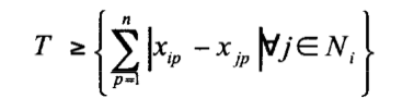
"one approach is to use Bayes' Rule and maximize the agreement between a model and the observed data"
Chapter 5 - Model Estimation, page 116
The Nature of Mathematical Modeling; Gershenfeld, Neil, Cambridge University Press 1999
Maximum Likelyhood Estimation -WIKIPEDIA-
Bayes' Rule -WIKIPEDIA-
01 Mar 17
Recognition Trials -- WA18
========================================================
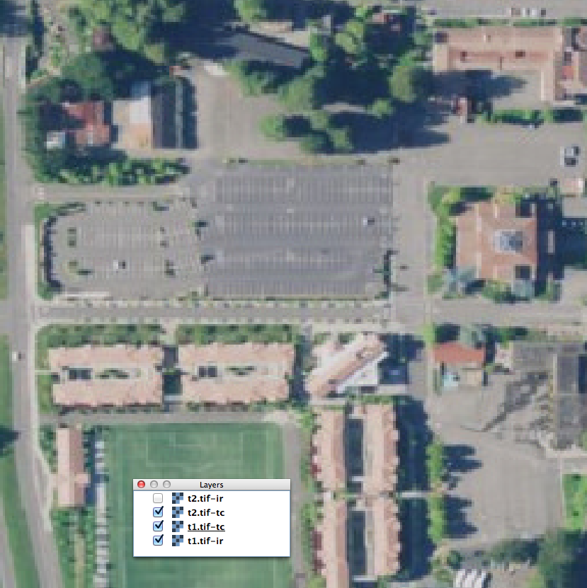
* prep for segmentation
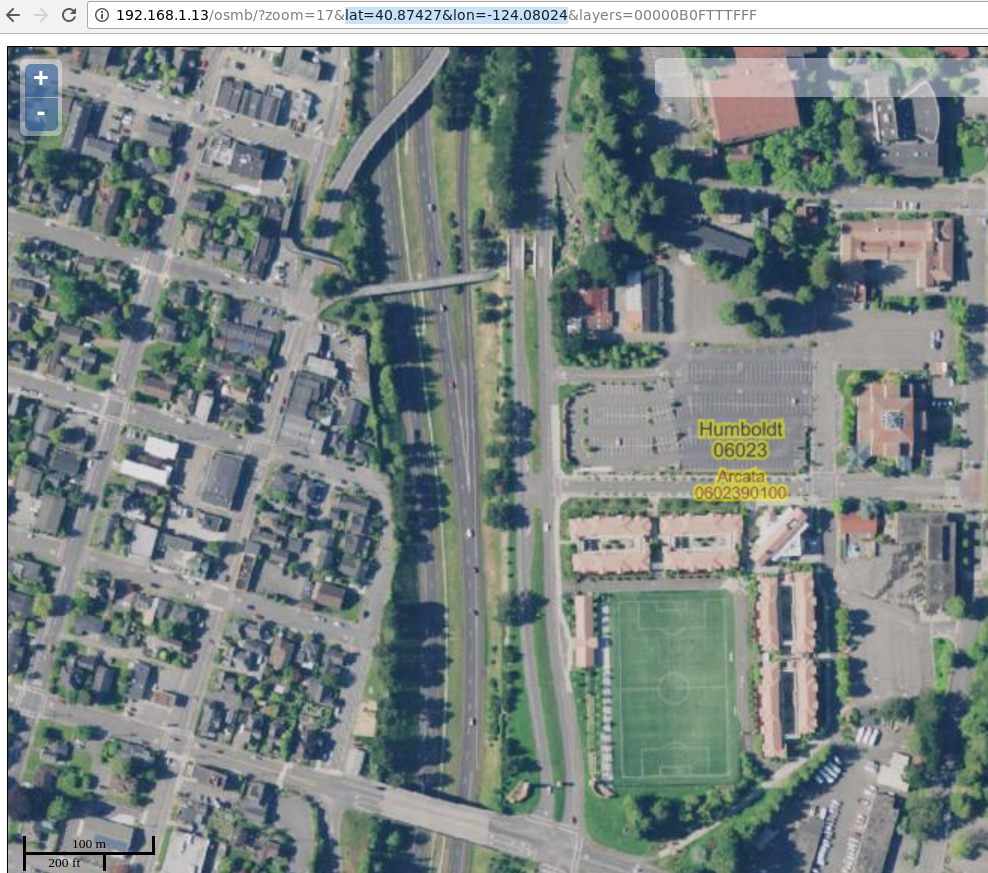
$ extract-image.py -o  /sand480/extractions_work/t2.tif -z 2 40.87427 -124.08024
/sand480/extractions_work/t2.tif-tc.tif
/sand480/extractions_work/t2.tif-ir.tif
- web visible results -LINK-
from Multiresolution Segmentation: an optimization approach for high quality multi-scale image segmentation -- Martin BAATZ und Arno SCHÄPE -LINK-
Design Goals: (for a generalized analysis method ed.)
Multiresolution: Objects of interest typically appear on different scales in an image simultaneously. The extraction of meaningful image objects needs to take into account the scale of the problem to be solved. Therefore the scale of resulting image objects should be free adaptable to fit to the scale of task.
Similar Resolution: Almost all attributes of image objects – color, texture or form -
are more or less scale-dependent. Only structures of similar size respectively scale
are of comparable quality. Hence the size of all resulting image objects should be of comparable scale.Reproducibility: Segmentation results should be reproducible
Universality: Applicable to arbitrary types of data and problems
Speed: Reasonable performance even on large image data sets
commentary: Let us focus here on the specific segmentation/extraction parameters (the "scale of the problem" is ambiguous in English, as it could refer to the total ambitions of the result set size). That is, the content of a scene by number of objects to be recognized, and the information in the scene, by measurable detail in the recorded bits. Both number of targets in a scene, and the detail available on each target, vary directly by scale -- aka zoom level.
The NAIP CA 2016 imagery has both IR and RGB layers, and with both layers, any reasonable desired "zoom level" is available, greater and lesser than the native resolution. Some questions here include:
* what combination of zoom levels + segmenting + analysis, within reasonable compute bounds given existing software and hardware, will yield accurate and consistent recognition for the size of the object we are searching for ?
* what segmentation detail will be most useful to identify likely targets?
* can we combine segmentation results from RGB and IR/Gray, in some way with our setup, to increase recognition? Do we need two training sets for ML, or can the two layers be combined ?
* if this search is focused on "big buildings", can we disregard completely "small buildings" footprints, like a typical residential, single-family home for example? Or, do we need the similarly shaped, but smaller footprint building in the result. Generally speaking, one building is more similar looking to other buildings, than to other kinds of features in the scene... except maybe parking lots !
* Can negative examples be used in a training set ? In other words, a segmented parking lot is "not a building".
-
We can think of "how big is a typical target, at a given scale" and "how many segments typically compose one target". Some explanation of these topics follows.
Consider a test area that is only 20% larger than a typical building of a certain class of interest. There is a huge amount of detail to match on, but, how many image analysis operations would it take to accomplish a survey ?
A counter-example is, analysis of an image at a zoom level such that there are one-hundred targets of interest. Each target is no longer a detailed polygon, but instead could be identified by the pattern of segments including the surrounding group, e.g. pixels for the building, its shadow, the road leading to it, cleared land around it, etc.
Can information from analysis at different scales, be combined in some rigorous way ? Does this overlap with combining non-segmentation data with segmentation data ? for example the presence of OSM polygons in a search area..
In case of boredom, a boot disk dropping off of its RAID is a remedy...
$ cat /proc/mdstat
Personalities : [raid1] [linear] [multipath] [raid0] [raid6] [raid5]
[raid4] [raid10]
md0 : active raid1 sdh[2] sda1[0]
244007744 blocks super 1.2 [2/1] [U_]
[====>................] recovery = 23.5% (57386432/244007744)
finish=53.0min speed=58672K/sec

unused devices:
Mask Files ?
- it seems there may be something missing in the extraction chain. There is an option in the gdal_translate code to "generate internal masks" but the way the processing chain is right now, the dot-msk files were left as a side product. This may need to change.
Map URLs as the Basis of Linking
The short-form of the map urls has zoom information and a center LatLon. This is useful at all steps in the analysis, from human to machine internals. Adapt the extract-image.py tool to use those zoom levels when reading NAIP imagery.
Search Notes:
* we think that "distance to a road" should be included in a preliminary search as a weight,
and that making effort eliminate whole areas from the search is worthwhile.
24 Feb 17
Recognition Trials -- California AB 802 Support
========================================================
James S. writes:
There is probably no documentation you haven't seen. The Python API source code is documentation
 of sorts. There is also a brief FAQ on imageseg.com

Honestly, different customers will either use or not use different parts for their specific
workflow. We lay it all out and let the integration happen at the customer end. As such there
are different pieces and you are welcome to use, disregard, or innovate on top of them.

You're certainly putting more software engineering effort into it than most.

The rank.py is optional for doing the shape comparison to determine the "goodness" of the
segmentation match to a ground truth shapefie. That embodies the gist of the Clinton paper.
Another potential post processing is supervised classification on the image stats.

Note automate.py and workflow.py modules that wrap the suggested workflow.

You are certainly welcome to build your own front end in Jupyter if that works for you. That
sounds like a good iterative/exploratory take on it. Some other customer in Africa just wanted
a GUI with four boxes. The land cover mapping customer in Mexico just did the whole country
at 10,0.5,0.5 and moved on. As I say, fit for purpose.
BIS Gui
- Threshold | 1-255 ? | close to 0 is "many colors in final"; 255 is "few colors in final"
- Shape Rate | [0.0,1.0] | 0 -> "many shapes"; "few shapes" -> 1.0
- Compact/Smoothness | [0.0,1.0] | 0 -> "compact; "spread" -> 1.0
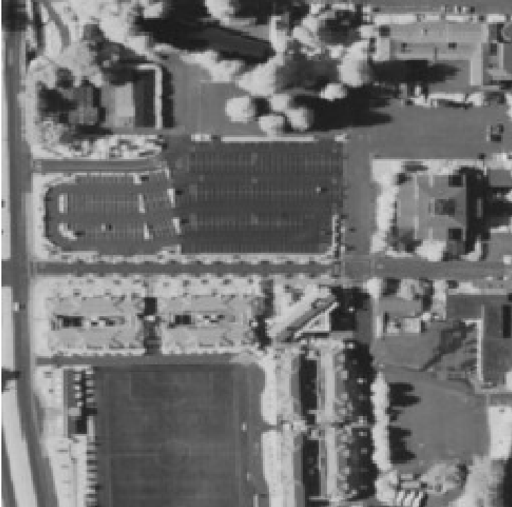
Base Example -IMG- Arcata_Ex0.png
A harsh first test; much detail, many similar objects.. ..
run in grayscale (IR) only
roughly 70 variations are produced (see exArcata dir)
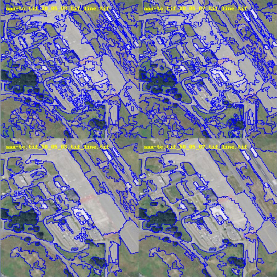
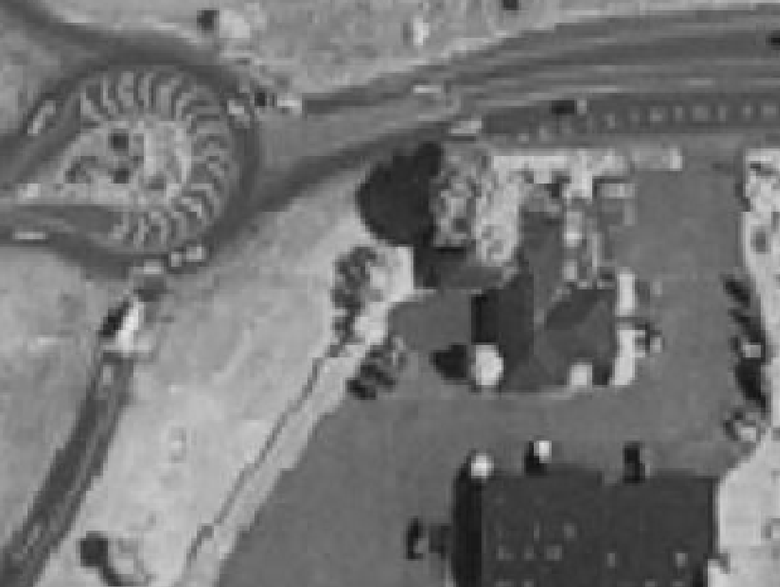
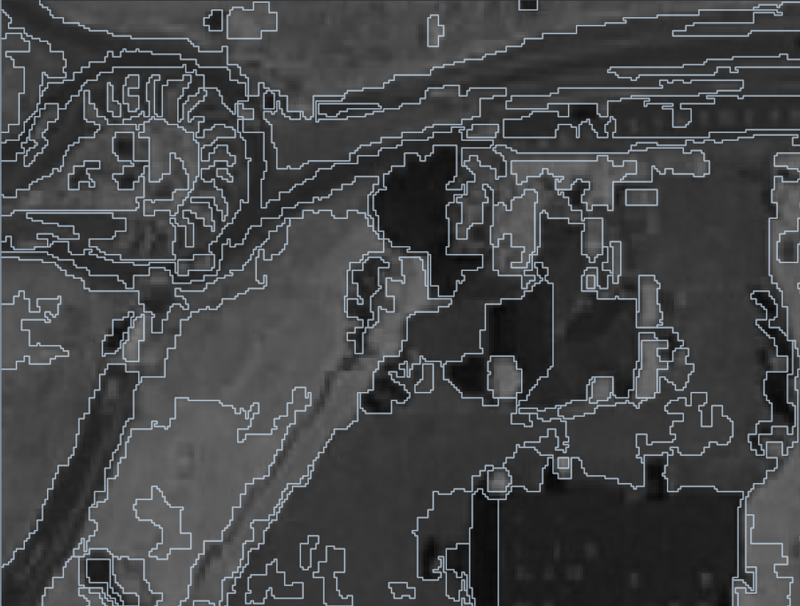
Example Vectorization using BIS:
Here is an IR layer image of Arcata, close up and shown at 50% intensity. Using the triple-inputs to BIS (threshhold, shape rate, smoothness) get a vector layer back. Do this twice, varying only the first parameter (threshhold). Notice how the same edges are picked in both cases, only more of them with a lower threshold.
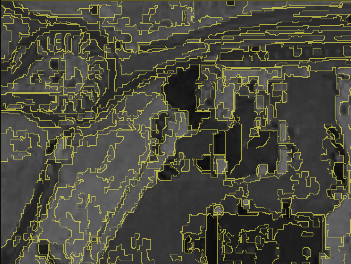
- ArcataEx0
- ArcataEx0 50_04_04
- ArcataEx0 30_04_04
Some observations: these vector result edges do follow the edge of change in pixel values, exactly. So the odd shapes of shadow and lighting, do carry through to the vector results. There appears to be no way for the vectorizing engine to estimate and resolve implied straight edges through shadows, for example. note: internally, BIS calls gdal.Polygonize() -LINK- to perform the vectorization.
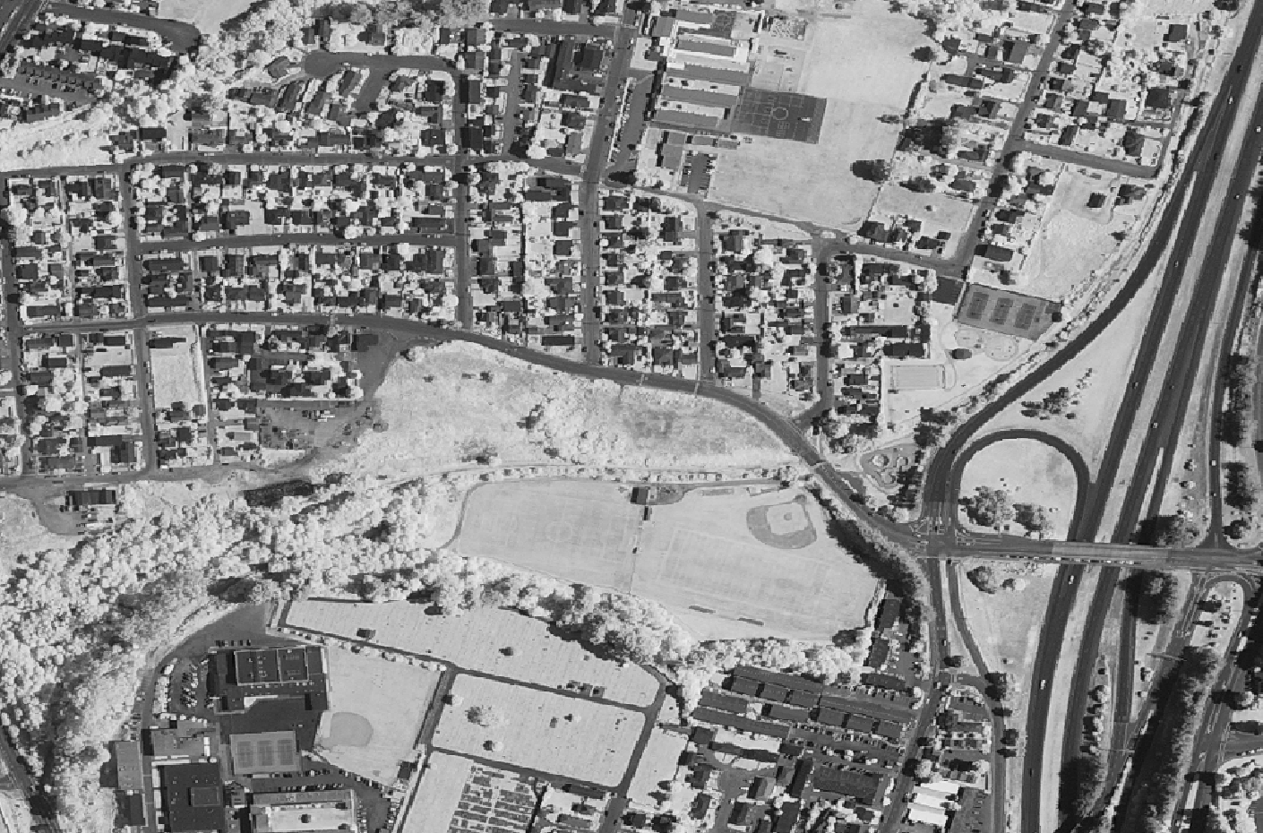
-- Some buildings in Chico, at zoom level 14 in Infrared (IR)
   /osmb/?zoom=14&lat=39.72545&lon=-121.80761&layers=0000BFFFTFFF
-- RGB Color, same scene in 2014
   /osmb/?zoom=14&lat=39.72545&lon=-121.80761&layers=000B0FFFTFFF
-- osm outlines, more to do !
   /osmb/?zoom=14&lat=39.72545&lon=-121.80761&layers=B0000FFFTTFF
Another form of output from the BIS engine is statistics available in a dot-csv file, each and every geometry is summed, including area in square units, mean luminance per pixel, and other statistical measures.. These statistics can be used to calibrate engine response in a feedback loop, using larger frameworks.
Questioning Machine Learning:
What is building and what is not building, in this image.
One question a ML process can answer is, is this (noisy thing) similar to this other noisy thing. Not the same to make a clean line in vector geometry! We may be asking several questions at once.. Where on the image is "building pixels" and where are not, is different than, provide a simple geometry representing each building. What is building, what is not building, in an image... is a different question than, show me a good representation of a building.
* developing a training set for supervised ML is work - a training set shows the learning system what a "right answer" is.. more than one hundred thousand, well-chosen examples is not uncommon in a training set. Developing the training set is not to be taken for granted.
* we have targets that do not change in life, but the view of them changes, due to weather, lighting, focus, image processing.
Example BIS Automation Run from the Command Line using IPython

$ cd /home/dbb/CEC_i7d/bis-2/bisapi-hamlin/bis-workd
$ ipython
Python 2.7.6 (default, Oct 26 2016, 20:30:19)
Type "copyright", "credits" or "license" for more information.

IPython 5.2.2 -- An enhanced Interactive Python.
...
In [3]: from automate import automate
...
In [4]:
    ...: files = automate('/wd4m/exArcata/Arcata_Ex0.png', t=[42,52,62,72,82],
    ...:   s=[0.5], c=[0.3,0.7],do_stats=True, do_colorize=False,
    ...:   do_train=False, do_classify=False, do_outline=True, do_lineup=True)
## -- BIS virtualenv Fresh Install --
ipython / jupyter / scipy / pyside  virtualenv re-install

    source /home/dbb/CEC_i7d/bis-2/bisenv/bin/activate bisenv
    pip install ipykernel
    python  -m ipykernel install --user --name bisenv --display-name "bisenv"
    pip install shapely fiona
    pip install scikit-image
    pip install numpy rasterio
    pip install pyproj cartopy
    pip install psycopg2
    pip install gdal   < - gives 2.1.3 which appears to work ok with 2.2dev


## - BIS working set of packages in virtualenv-
##
(bisenv) dbb@i7d:~/CEC_i7d/bis-2/bisapi-hamlin/bis-workd$ pip freeze
affine==2.0.0.post1  Cartopy==0.14.2   Fiona==1.7.3    GDAL==2.1.3
ipykernel==4.5.2    ipython==5.2.2    ipython-genutils==0.1.0
jupyter-client==4.4.0    jupyter-core==4.3.0
matplotlib==2.0.0    numpy==1.12.0    Pillow==4.0.0    psycopg2==2.6.2    ...
pyproj==1.9.5.1    pyshp==1.2.10    PySide==1.2.4    ...
rasterio==0.36.0    scipy==0.18.1    Shapely==1.5.17    ...
six==1.10.0    subprocess32==3.2.7    tornado==4.4.2    ...

## Fiona CLI tool - (no PG driver)
$fio env
  ...
  ESRI Shapefile (modes 'r', 'a', 'w')
  GPKG (modes 'r', 'w')
  GPSTrackMaker (modes 'r', 'a', 'w')
  GPX (modes 'r', 'a', 'w')
  GeoJSON (modes 'r', 'w')
  OpenFileGDB (modes 'r')
  ...
i7d Disk Updates:
* naip-fetch2/process-doqqs.py
- add dir /sand480/tmp
Google Search \ filetype:pdf inurl:asprs object
http://wiki.openstreetmap.org/wiki/OpenSolarMap
https://github.com/opensolarmap/solml
BIS Test 2
visually picked an area in IR; important variables: zoom level, color/gray; composition
/osmb/?zoom=17&lat=40.8835&lon=-124.08918&layers=0000BTFFFFFF -LINK-
Use the DOQQ labels layer in the map to find the filename of the right image on disk; picked out a subset using rio tool
rio info final-ir/m_4012408_sw_10_1_20140607.tif
take one-hundredth of a degree in each direction, from some buildings
$ rio clip input.tif output.tif --bounds xmin ymin xmax ymax

  --bounds #(-124.087-0.01) (40.878-0.01) (-124.087+0.01)   (40.878+0.01)

rio clip final-ir/m_4012408_sw_10_1_20140607.tif /tmp/work1.tif --bounds -124.097 40.868 -124.077 40.888
try expanding the file with gdal to 2x resolution
gdal_translate -outsize 200% 0 /tmp/work1.tif /tmp/work2.tif

   ...

-rw-rw-r-- 1 dbb dbb 24M Feb 20 19:09 work2.tif

-rw-rw-r-- 1 dbb dbb 6.0M Feb 20 19:00 /tmp/work1.tif
but, the image result looks exactly the same, just 4x the size on disk.
onward -- go to BIS work dir
dbb@i7d:~/CEC_i7d/bis-2/bisapi-hamlin/bis-workd$ source /home/dbb/CEC_i7d/bis-2/bisenv/bin/activate bisenv

(bisenv) dbb@i7d:~/CEC_i7d/bis-2/bisapi-hamlin/bis-workd$ ipython
In [1]: from automate import automate
files = automate('/tmp/work1.tif', t=[42,48,54,60,72], s=[0.1,0.2,0.4,0.6,0.9], c=[0.5],do_stats=True, do_colorize=False, do_train=False, do_classify=False, do_outline=True, do_lineup=True)
CRASH in outline burn()
repeat with do_outline=False
also note, turn off stats if they are not being used
files = automate('/tmp/work1.tif', t=[42,48,54,60,72], s=[0.1,0.2,0.4,0.6,0.9], c=[0.5],do_stats=False, do_colorize=False, do_train=False, do_classify=False, do_outline=False, do_lineup=True)
automate() invokes the engine five times, each time thresholds are evaluated from one to the largest threshhold in t, and len(t) number of outputs are emitted. A run in this example allocates 12GB of RAM.... about 40 seconds per run.. 5 runs with 5 outputs each, in this example.
example output:


New Data - NAIP CA 2016 0.6m
copying ...
$ /naip_16/d2/naip/ca_60cm_2016/40124$ ls -lh m_4012408_sw_10_h_20160528.tif
-rwxrwxrwx 2 root root 439M Sep 29 04:22 m_4012408_sw_10_h_20160528.tif

##-- test area in Arcata, CA
rio info /naip_16/d2/naip/ca_60cm_2016/40124/m_4012408_sw_10_h_20160528.tif
{"count": 4, "crs": "EPSG:26910", "colorinterp": ["red", "green", "blue", "undefined"], "interleave": "pixel", "dtype": "uint8", "driver": "GTiff", "transform": [0.6, 0.0, 405054.0, 0.0, -0.6, 4532580.0], "lnglat": [-124.0937491743777, 40.90625190492096], "height": 12180, "width": 9430, "shape": [12180, 9430], "tiled": false, "res": [0.6, 0.6], "nodata": null, "bounds": [405054.0, 4525272.0, 410712.0, 4532580.0]}
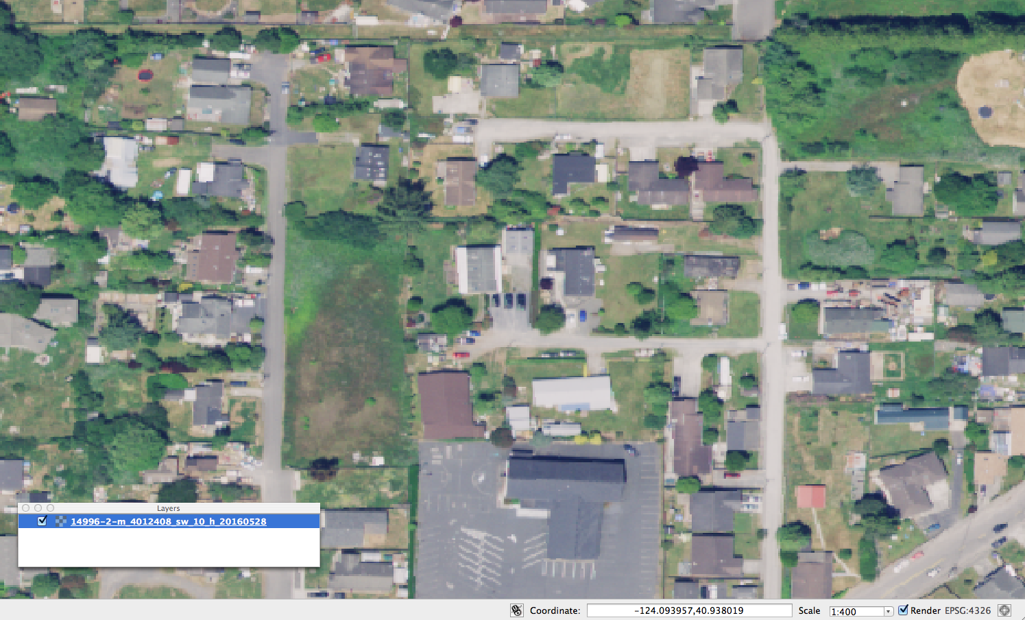
NAIP California 2016, 0.6 meter per pixel, compressed JPEG YCbCr in 4326
Prioritizing LA County in NAIP 2016
auth_buildings=#
  update doqq_processing as a
    set priority=6 from tl_2016_us_county b, naip_3_16_1_1_ca c
      where
        b.statefp='06' and b.countyfp='037' and
        st_intersects(b.geom, c.geom) and a.doqqid=c.gid;
Feb 15 -ARCHIVE-
Jan 17 -ARCHIVE-
2016 ARCHIVE Main -LINK-