darkblue blog

In preparing for an upcoming Datathon, a column of data in PostgreSQL numeric format needed formatting for presentation. “Intersection Count” intersection_density_sqkm is a count of street intersections per unit area – a quick way to measure density of the built environment. A table of grid cells (covering the nine-county San Francisco Bay Area) that the column comes from consists of roughly 814,000 cells. How to quickly characterize the data contents? Use SQL and the psql quantile extension to look at ranges, with and without the zeroes.
 

SELECT 
   min(intersection_density_sqkm), 
    quantile(intersection_density_sqkm,ARRAY[0.02,0.25,0.5,0.75,0.92]), 
   max(intersection_density_sqkm) 

 FROM uf_singleparts.ba_intersection_density_sqkm

-[ RECORD 1 ]-----------------------------------------------------------------------------
min      | 0.0
quantile | {0.0, 0.0, 0.683937...,3.191709...,25.604519...}
max      | 116.269430...

Psql extension quantile takes as arguments a column name and an ARRAY for N positional elements by percentage, e.g. above

---

How Many Gridcells Have Non-zero Data ?

select count(*) from ba_intersection_density_sqkm;
count => 814439

select count(*) from ba_intersection_density_sqkm where intersection_density_sqkm <> 0;
count => 587504

 Select stats on non-zero data

 SELECT 
   min(intersection_density_sqkm), 
    quantile(intersection_density_sqkm,ARRAY[0.02,0.25,0.5,0.75,0.92]), 
   max(intersection_density_sqkm) 

 FROM uf_singleparts.ba_intersection_density_sqkm

 where intersection_density_sqkm <> 0;

-[ RECORD 1 ]-----------------------------------------------------------------------------
min      | 0.227979...
quantile | {0.227979...,0.455958...,1.367875...,7.751295...,31.461139...}
max      | 116.269430...

 
and, what does the high-end of the range look like ? Use SQL for a quick visual inspection for either outliers or smooth transitions:

SELECT intersection_density_sqkm 
FROM ba_intersection_density_sqkm 
 ORDER BY  intersection_density_sqkm   desc limit 12;

 intersection_density_sqkm 
---------------------------
      116.2694300518134736
      115.5854922279792768
      115.3575129533678764
      115.1295336787564760
      114.9015544041450756
      114.9015544041450756
      114.4455958549222792
      113.7616580310880824
      112.6217616580310892
      112.6217616580310892
      112.1658031088082884
      112.1658031088082884

 

So, recall that a natural log e of 1.0 is 0; a natural log of 116 is slightly over 4.75; a natural log of a number less than 1 is a negative number. To simplify the range for visualization, add a float column called data, set the new data column to the natural log of (intersection_density_sqkm + 1); use a simple multiply-then-divide technique to limit the precision to two digits (screenshot from an IPython Notebook session using psycopg2).

 select quantile(data,ARRAY[0.02,0.25,0.5,0.75,0.92]) from ba_intersection_density_sqkm;
  { 0, 0, 0.52, 1.43, 3.28 }

SELECT
  min(data), 
    quantile(data,ARRAY[0.02,0.25,0.5,0.75,0.92]), 
  max(data) 
FROM ba_intersection_density_sqkm
WHERE data <> 0;

 min  |          quantile          | max  
------+----------------------------+------
 0.21 | {0.21,0.38,0.86,2.17,3.48} | 4.76
(1 row)

 

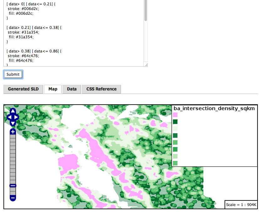
Final Results in GeoServer 2.5 CSS styler:

ps- a full sequential scan on this table takes about four seconds, on a Western Digital Black Label 1TB disk, ext4 filesystem, on Linux.