OSGeo.org collaborated to show this banner prominently
on September 20th, 2019


OSGeo.org collaborated to show this banner prominently
on September 20th, 2019

.. the hands of time move slowly sometimes. I just got this email:
Dear Dav Clark, Aaron Culich, Brian M Hamlin, and Ryan Lovett,
Your paper from the 13th Python in Science Conference titled “BCE: Berkeley’s Common Scientific Compute Environment for Research and Education” has been assigned the DOI 10.25080/Majora-14bd3278-002. Please use this DOI when providing citations for your paper, following the guidelines here: https://www.crossref.org/display-guidelines/#full
Yours,
Dillon Niederhut, on behalf of:
Stéfan van der Walt
James Bergstra
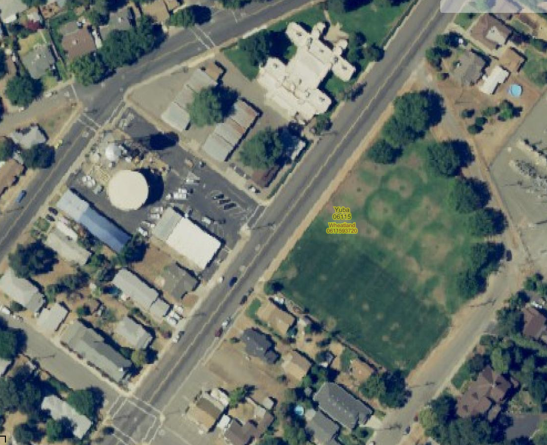
Running 11,000 DOQQs through a processing pipeline – so far, so good !
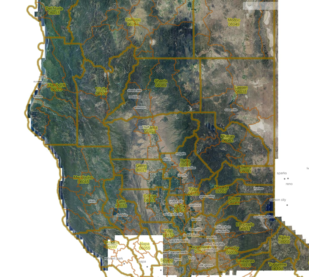
Details at 0.6 meters per pixel:
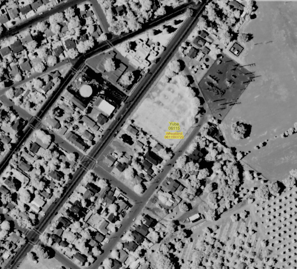
Prioritize LA, for Today
auth_buildings=#
  update doqq_processing as a
    set priority=6 from tl_2016_us_county b, naip_3_16_1_1_ca c
      where
        b.statefp='06' and b.countyfp='037' and
        st_intersects(b.geom, c.geom) and a.doqqid=c.gid;

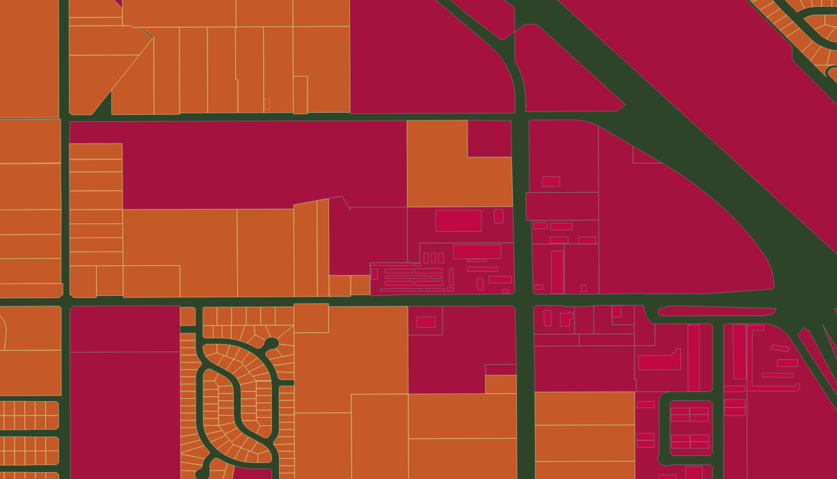
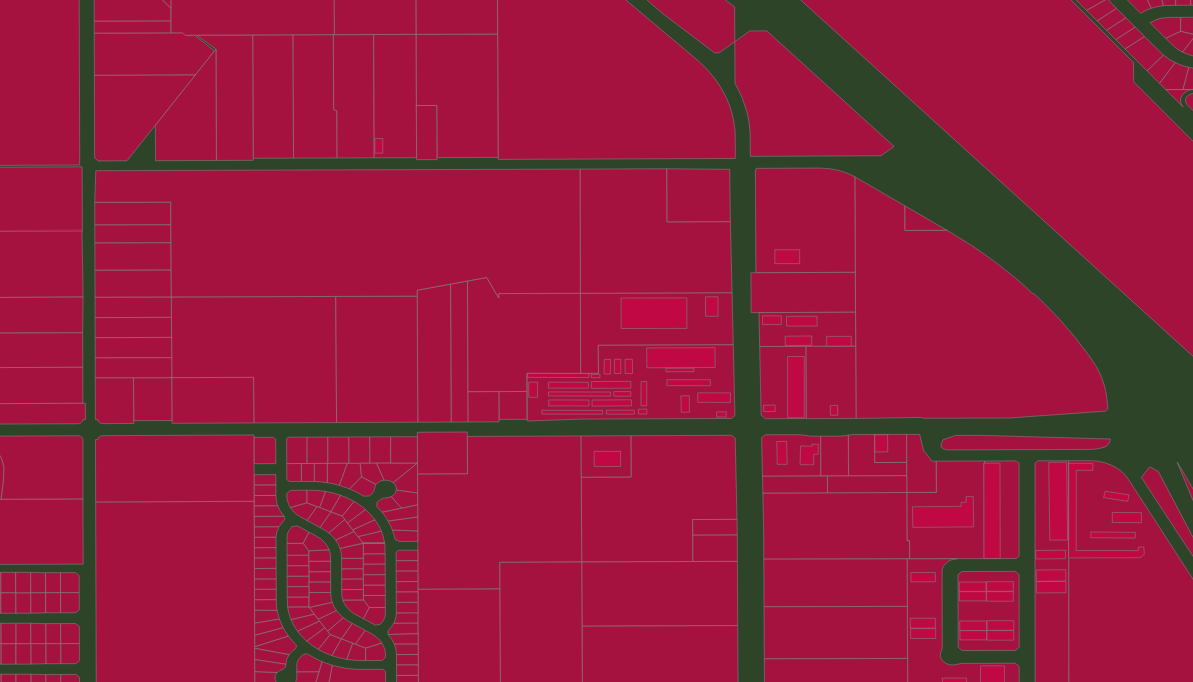
In Openstreetmap US, California Fresno area, a controversial [0] series of imports of legal property records (aka PARCEL) are mixed in with other POLYGONS. Many various POLYGON in Fresno now share the tag landuse=residential, both the PARCEL legal records and real building footprint POLYGON, as well as various others. After reviewing the wiki talk page, relevant discussions, and discussing online briefly, this post looks at the OSM context; estimates the extent of these imports by examining similar, nearby areas; compares the OSM records to actual current PARCEL records; proposes a deletion criteria and finally, examines the extent of the proposed deletion.
[0] changeset/26356220 * changeset/26357831
OSM Wiki on Parcels -LINK- -TALK-
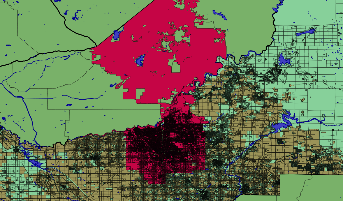
Context: Fresno County is big — but the real-world residential areas are confined almost entirely to the City of Fresno.
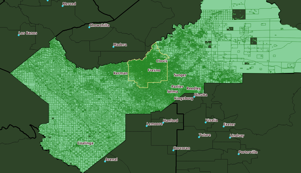
Q. What tag 'landuse' values are present in County Subdivision Fresno?

 151670 | residential
   6644 | commercial
   6463 | NULL
   3859 | industrial
    706 | farm
    574 | vineyard
    498 | orchard
    453 | meadow
    109 | garages

less than 100:
  basin,farmyard,recreation_ground,grass,farmland,religious,cemetery,retail,
  quarry,reservoir,railway,landfill,construction,institutional
Next, expand the query to the entire five-county region
Q. What tag 'landuse' values are present in the five county area
-- Kings, Madera, Tulare, Kern, Fresno

 207902 | NULL
 203000 | residential
  11697 | commercial
   7054 | farm
   6679 | orchard
   5941 | industrial
   5251 | vineyard
   5029 | meadow
   2475 | farmland
   1980 | farmyard
    885 | grass

less than 300:
   garages,cemetery,recreation_ground,basin,quarry,reservoir,religious,retail
  forest,scrub,military,landfill,railway,pond,greenhouse_horticulture,construction
So, 150,000 of the 200,000 landuse=residential tagged POLYGONs in a five-county area, are in just the Fresno City CCD.
Attribution On inspection, a large number of likely PARCEL records in Fresno, carry an attribution tag with one of several recognizable values: Caltrans (4), FMMP (3) and Fresno_County_GIS.
example data:
 "type"=>"multipolygon", "landuse"=>"vineyard", "attribution"=>"Fresno_County_GIS"
 "crop"=>"field_cropland", "type"=>"multipolygon", "landuse"=>"farm", "attribution"=>"Fresno_County_GIS"
 "crop"=>"field_cropland", "type"=>"multipolygon", "landuse"=>"farm", "attribution"=>"Fresno_County_GIS"
 "crop"=>"native_pasture", "type"=>"multipolygon", "landuse"=>"meadow", "attribution"=>"Fresno_County_GIS"
 "crop"=>"native_pasture", "type"=>"multipolygon", "landuse"=>"meadow", "attribution"=>"Fresno_County_GIS"
 "type"=>"multipolygon", "landuse"=>"vineyard", "attribution"=>"Fresno_County_GIS"
 "crop"=>"field_cropland", "type"=>"multipolygon", "landuse"=>"farm", "attribution"=>"Fresno_County_GIS"
 "type"=>"multipolygon", "landuse"=>"vineyard", "attribution"=>"Fresno_County_GIS"
 "crop"=>"field_cropland", "type"=>"multipolygon", "landuse"=>"farm", "attribution"=>"Fresno_County_GIS"
 "type"=>"multipolygon", "trees"=>"orange_trees", "landuse"=>"orchard", "attribution"=>"Fresno_County_GIS"
 "type"=>"multipolygon", "landuse"=>"residential", "lot_type"=>"single family residential properties", "other_use"=>"S", "attribution"=>"Fresno_County_GIS", "primary_use"=>"000", "secondary_use"=>"VLM"
 "type"=>"multipolygon", "wood"=>"mixed", "landuse"=>"farm", "natural"=>"wood", "attribution"=>"Fresno_County_GIS"
 "type"=>"multipolygon", "landuse"=>"vineyard", "attribution"=>"Fresno_County_GIS"
 "type"=>"multipolygon", "landuse"=>"orchard", "attribution"=>"Fresno_County_GIS"
Detailed counts in Fresno County and the Fresno CCD
-- Fresno County:  geoid  06019 / tl_2016_us_county
241860 - all multipolygons
231624 - tag landuse
196017 - tag landuse = 'residential'
230685 - tag 'attribution'
230612 - tag 'attribution' ~* 'GIS'
----------------------------------------------------
-- Fresno CCD:   geoid   0601991080
171200 - all multipolygons
164737 - tag landuse
151670 - tag landuse = 'residential'
166163 - tag 'attribution'
166147 - tag 'attribution' ~* 'GIS'
----------------------------------------------------
-- Fresno County outside of Fresno CCD (derived)
 70660 - all multipolygons   (241860 - 171200)
 66887 - tag landuse         (231624 - 164737)
 44347 - tag landuse = 'residential'  (196017 - 151670)
 64465 - tag 'attribution' ~* 'GIS'   (230612 - 166147)
Qry - count the occurances of attribution 'GIS'   AND
  landuse = 'residential'; area Fresno County, by cousub
           name           | count
--------------------------+--------
 Caruthers-Raisin City    |   1400
 Fresno                   | 150681
 Kerman                   |   4093
 Reedley                  |   5967
 Mendota                  |   1779
 San Joaquin-Tranquillity |   1030
 Coalinga                 |   2528
 Firebaugh                |   1152
 Orange Cove              |   1579
 Kingsburg                |   3557
 Huron                    |     87
 Fowler                   |   1527
 Sierra                   |    963
 Parlier-Del Rey          |   2633
 Sanger                   |   7796
 Riverdale                |   1208
 Laton                    |    599
 Selma                    |   6221
Compare current parcel data (670 records) to OSM multipolygon with tag landuse=residential (350 records), in a sample Fresno blockgroup ('060190045051')
BBOX="-119.7994,36.8084,-119.7903,36.8229"


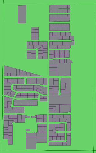
This looks promising: take all OSM multipolygons marked landuse=residential, then remove WHERE tag attribution exists AND tag building does not exist …

Some Links:
https://help.github.com/articles/mapping-geojson-files-on-github/
-- County of Fresno, subdivision Fresno geoid = '0601991080'
-- multipolygons m is a raw dot-pbf import of OSM
-- Qry - Show all landuse tags and a count of occurances
-- area: Fresno CCD
--
select count(*), all_tags -> 'landuse'
FROM multipolygons m, tl_2016_06_cousub cs
WHERE
cs.geoid = '0601991080' AND
st_intersects( m.wkb_geometry, cs.geom)
GROUP BY all_tags -> 'landuse'
ORDER BY all_tags -> 'landuse';
/* count | landuse tag
--------+-------------------
48 | basin
11 | cemetery
6644 | commercial
1 | construction
706 | farm
24 | farmland
43 | farmyard
109 | garages
28 | grass
3859 | industrial
1 | institutional
1 | landfill
453 | meadow
498 | orchard
2 | quarry
1 | railway
37 | recreation_ground
19 | religious
2 | reservoir
151670 | residential
6 | retail
574 | vineyard
6463 |
*/
--=====================================================
--
-- Kern County - FIPS 029
-- Fresno County - FIPS 019
--
-- Qry - Show CCDs and a count of tag landuse = 'residential'
-- area: Fresno County, Kern County
--
select count(*), (cs.geoid, cs.name, cs.countyfp)
FROM multipolygons m, tl_2016_06_cousub cs
WHERE
cs.countyfp IN ( '019', '029' ) AND
all_tags -> 'landuse' = 'residential' AND
st_intersects( m.wkb_geometry, cs.geom)
GROUP BY (cs.geoid, cs.name, cs.countyfp)
ORDER BY (cs.geoid, cs.name, cs.countyfp) ;
/*
1408 | (0601990390,"Caruthers-Raisin City",019)
2558 | (0601990530,Coalinga,019)
1170 | (0601991000,Firebaugh,019)
1541 | (0601991060,Fowler,019)
151670 | (0601991080,Fresno,019)
...............
60 | (0602990130,Arvin-Lamont,029)
724 | (0602990180,Bakersfield,029)
................
1096 | (0602993320,Tehachapi,029)
188 | (0602993570,Wasco,029)
715 | (0602993635,"West Kern",029)
*/
--==================================================
--
-- Qry - Show all landuse tags and a count of occurances
-- area: Fresno County, Kern County
----
select count(*), all_tags -> 'landuse'
FROM multipolygons m, tl_2016_06_cousub cs
WHERE
cs.countyfp IN ( '019', '029' ) AND
st_intersects( m.wkb_geometry, cs.geom)
GROUP BY all_tags -> 'landuse'
ORDER BY all_tags -> 'landuse';
/* count | landuse tag
--------+-------------------------
1 | aerodrome
83 | basin
54 | cemetery
11107 | commercial
1 | conservation
1 | construction
5160 | farm
2426 | farmland
1034 | farmyard
5 | forest
268 | garages
885 | grass
1 | greenhouse_horticulture
5830 | industrial
1 | institutional
3 | landfill
3318 | meadow
4 | military
6519 | orchard
45 | quarry
3 | railway
86 | recreation_ground
19 | religious
19 | reservoir
201341 | residential
13 | retail
16 | scrub
5225 | vineyard
203195 |
*/
--===================================================
--
-- Qry - Show all landuse tags and a count of occurances
-- area: Bakersfield city, Kern County (similar to Fresno city )
--
select count(*), all_tags -> 'landuse'
FROM multipolygons m, tl_2016_06_place p
WHERE
p.namelsad = 'Bakersfield city' AND
st_intersects( m.wkb_geometry, p.geom)
GROUP BY all_tags -> 'landuse'
ORDER BY all_tags -> 'landuse';
/* count | landuse tag
--------+-------------------
4 | cemetery
687 | commercial
78 | farm
3 | farmland
23 | farmyard
836 | grass
261 | industrial
52 | meadow
18 | orchard
1 | railway
8 | recreation_ground
710 | residential
16 | scrub
119669 |
*/
--===================================================
--
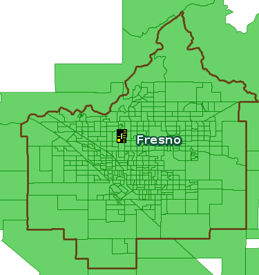
-- Qry - Show all landuse tags and a count of occurances
-- area: Fresno City
--
--
select count(*), all_tags -> 'landuse'
FROM multipolygons m, tl_2016_06_place p
WHERE
p.namelsad = 'Fresno city' AND
st_intersects( m.wkb_geometry, p.geom)
GROUP BY all_tags -> 'landuse'
ORDER BY all_tags -> 'landuse';
/* count | landuse tag
--------+-------------------
25 | basin
5 | cemetery
5523 | commercial
1 | construction
67 | farm
4 | farmland
4 | farmyard
65 | garages
12 | grass
2410 | industrial
1 | landfill
268 | meadow
45 | orchard
1 | railway
26 | recreation_ground
19 | religious
1 | reservoir
105930 | residential
5 | retail
15 | vineyard
5192 |
*/
![]()
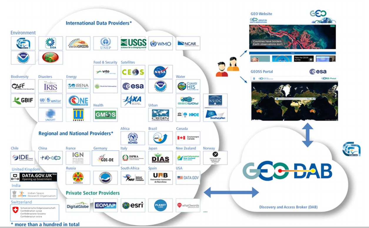
The Group On Earth Observation System of Systems (GEOSS) plenary conference was held in November of 2016.
2017 Work Plan -LINK-
Earth System Grid -PAGE-
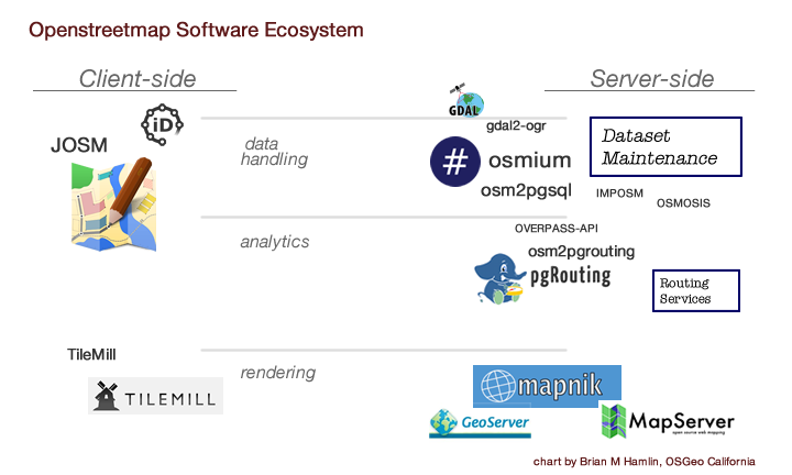
There is a non-obvious relationship of big engines like Mapnik, and the rest of Openstreetmap activity. While building OSGeo-Live v10, I am trying to make sense of “the whole of openstreetmap software” — to make a map of it, so to speak.. but a map of logical groupings, by purpose, and weighted by popularity and utility. Server-side to client-side is represented as one spectrum, right to left.. and then separate activity classes, like the difference between data pipelines for maintenance, rendering, and more recently, analysis.. then the nouns of the actual software projects, some of which are quite large, like Mapnik.
related links:
http://wiki.openstreetmap.org/wiki/Develop#How_the_pieces_fit_together
Mapnik: main site; OSM wiki page;wiki; tutorial; repo; python interfaces; python-mapnik quickstart
OSMIUM repo; pyosmium; and other OSM Code
osm2pgsql repo and a tutorial
Imposm3 repo and tutorial
OSM Node One http://www.openstreetmap.org/node/1
OSM dot-org Internal Git https://git.openstreetmap.org/
OSM Packaging in Debian -blends- -ref-
OSM TagInfo language example
US TIGER Data
A representative example of US Census Bureau TIGER data, integrated into OSM. -Here-
OSMBuildings
Sonoma State University in osmbuildings
osmlab labuildings gitter channel
OSM Wiki – Multipoygons -link-
OSM-Analytics
>-here- presented by mikel maron and jennings anderson at SOTM-US in this video Odd thing here may be, that the “unit of analysis is the tile” .. so, in a twist, the delivery of the graphics, becomes the unit of analytics. MapBox blog post on osm-qa tiles
Overpass-Turbo
Openstreetmap Wiki Overpass-turbo
OSM Future Directions have been brewing for a long time
Other Notable Resources
3rd Party OSM WMTS OWS Service via MapProxy
Wikimedia Foundation Maps https://www.mediawiki.org/wiki/Maps
Omniscale Gmbh and Co. KG, OSM https://osm.omniscale.de
Overpress Express http://overpass-turbo.eu/
OSM Software Watchlist -here-
OSM Geometry Inspector -link-
OpenSolarMap -hackpad- http://opensolarmap.org -Github-
http://2016.stateofthemap.org/2016/opensolarmap-crowdsourcing-and-machine-learning-to-classify-roofs/
OSM Basemaps -LINK-
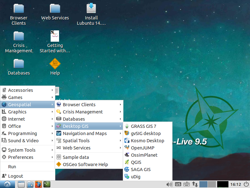 The OSGeo Community has announced immediate availability of the OSGeo-Live reference distribution of geospatial open-source software, version 9.5. OSGeo-Live is available now as both 32-bit and 64-bit .iso images, as well as a 64-bit Virtual Machine (VM), ready to run. Users across the globe can depend on OSGeo-Live, which includes overview and introductory examples for every major software package on the disk, translated into twelve languages. LINK
New Applications:
• Project Jupyter (formerly the IPython Notebook) with examples
• istSOS – Sensor Observation Service
• NASA World Wind – Desktop Virtual Globe
Twenty-two geospatial programs have been updated to newer versions, including:
• QGIS 2.14 LTR with more than one hundred new features added or improved since the last QGIS LTR release (version 2.8), sponsored by dozens of geospatial data providers, private sector companies and public sector governing bodies around the world.
• MapServer 7.0 with major new features, including complex filtering being pushed to the database backends, labeling performance and the ability to render non-latin scripts per layer. See the complete list of new features
• Cesium JavaScript library for world-class 3D globes and maps
• PostGIS 2.2 with optional SFCGAL geometry engine
• GeoNetwork 3.0
Analytics and Geospatial Data Science:
• R geostatistics
• Python reference libraries including Iris, SciPy, PySAL, geoPandas
OSGeo-Live is a self-contained bootable USB flash drive, DVD and Virtual Machine, pre-installed with robust open source geospatial software, which can be trialled without installing any software.
• Over 50 quality geospatial Open Source applications installed and pre-configured
• Free world maps and sample datasets
• Project Overview and step-by-step Quickstart for each application
• Lightning presentation of all applications, along with speaker’s script
• Overviews of key OGC standards
• Translations to multiple languages
• Based upon the rock-solid Lubuntu 14.04 LTS GNU/Linux distribution, combined with the light-weight LXDE desktop interface for ease of use.
Homepage: http://live.osgeo.org
Download details: http://live.osgeo.org/en/download.html
Post release glitches collected here: http://wiki.osgeo.org/wiki/Live_GIS_Disc/Errata/9.5
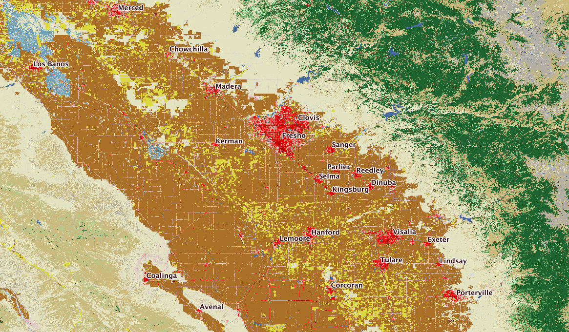
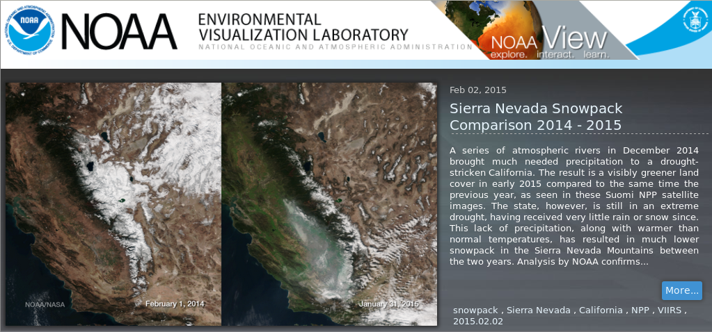
For those that have been following the Climate Change story over the years, this satellite imagery tells a story quite vividly.. no modelling uncertainty involved.
![]()
At a minimum, suffice it to say I participated online in roughly twelve hours of lecture and lab on Nov 20 and 21, 2014 at AmpCamp 5 (I also attended one in Fall 2012). I put an emphasis on python, IPython Notebook, and SQL.
Once again this year, the camp mechanics went very smoothly — readable and succinct online exercises; Spark docs; Spark python, called pyspark is advancing, although some interfaces may not be available to python yet; Spark SQL appears to be useable.
To setup on my own Linux box, I unzipped the following files:
ampcamp5-usb.zip ampcamp-pipelines.zip training-downloads.zip
The resulting directories provided a pre-built Spark 1.1
Using Scala version 2.10.4 (OpenJDK 64-Bit Server VM, Java 1.7.0_65)
The Lab exercises are almost all available as both Scala and python. Tools to do the first labs:
$SPARK_HOME/bin/spark-shell $SPARK_HOME/bin/pyspark
and for extra practice
$SPARK_HOME/bin/spark-submit $SPARK_HOME/bin/run-example
IPython Notebook
An online teaching assistant (TA) suggested a command line to launch the Notebook – here are my notes:
##-- TA suggestion
IPYTHON_OPTS="notebook --pylab inline" ./bin/pyspark --master "local[4]"
##-- a server already setup with a Notebook, options
--matplotlib inline --ip=192.168.1.200 --no-browser --port=8888
##-- COMBINE
IPYTHON_OPTS="notebook --matplotlib inline --ip=192.168.1.200 --no-browser --port=8888" $SPARK_HOME/bin/pyspark --master "local[4]"
The IPython Notebook worked ! Lots of conveniences, interactivity and viz potential immediately available against the pyspark environment. I created several Notebooks in short order, to test and explore, for example SQL.
The SQL exercise reads data from a format new to me, called Parquet
Part 1.2
After rest and recuperation, I wanted to try python in the almost-ready Spark 1.2 branch. It turned out to build and run easily. First get the spark code:
https://github.com/apache/spark/tree/branch-1.2
make sure maven is installed on your system, then run
./make-distribution.sh
. Afterwards, I set $SPARK_HOME to this directory, and launched IPython Notebook again. All the examples and experiments I had built worked without modification ! Success.
Other Links
http://databricks.com/blog/2014/03/26/spark-sql-manipulating-structured-data-using-spark-2.html
http://spark-summit.org/2014/training
https://github.com/amplab-extras
http://www.planetscala.com/
experimental
https://github.com/ooyala/spark-jobserver