Skip to content

Numeric Stats on Bay Area Intersection Counts

pg_logo

In preparing for an upcoming Datathon, a column of data in PostgreSQL numeric format needed formatting for presentation. “Intersection Count” intersection_density_sqkm is a count of street intersections per unit area – a quick way to measure density of the built environment. A table of grid cells (covering the nine-county San Francisco Bay Area) that the column comes from consists of roughly 814,000 cells. How to quickly characterize the data contents? Use SQL and the psql quantile extension to look at ranges, with and without the zeroes.
 

SELECT 
   min(intersection_density_sqkm), 
    quantile(intersection_density_sqkm,ARRAY[0.02,0.25,0.5,0.75,0.92]), 
   max(intersection_density_sqkm) 

 FROM uf_singleparts.ba_intersection_density_sqkm
-[ RECORD 1 ]-----------------------------------------------------------------------------
min      | 0.0
quantile | {0.0, 0.0, 0.683937...,3.191709...,25.604519...}
max      | 116.269430...

Psql extension quantile takes as arguments a column name and an ARRAY for N positional elements by percentage, e.g. above


How Many Gridcells Have Non-zero Data ?

select count(*) from ba_intersection_density_sqkm;
count => 814439

select count(*) from ba_intersection_density_sqkm where intersection_density_sqkm <> 0;
count => 587504

 Select stats on non-zero data

 SELECT 
   min(intersection_density_sqkm), 
    quantile(intersection_density_sqkm,ARRAY[0.02,0.25,0.5,0.75,0.92]), 
   max(intersection_density_sqkm) 

 FROM uf_singleparts.ba_intersection_density_sqkm

 where intersection_density_sqkm <> 0;
-[ RECORD 1 ]-----------------------------------------------------------------------------
min      | 0.227979...
quantile | {0.227979...,0.455958...,1.367875...,7.751295...,31.461139...}
max      | 116.269430...

 
and, what does the high-end of the range look like ? Use SQL for a quick visual inspection for either outliers or smooth transitions:

SELECT intersection_density_sqkm 
FROM ba_intersection_density_sqkm 
 ORDER BY  intersection_density_sqkm   desc limit 12;

 intersection_density_sqkm 
---------------------------
      116.2694300518134736
      115.5854922279792768
      115.3575129533678764
      115.1295336787564760
      114.9015544041450756
      114.9015544041450756
      114.4455958549222792
      113.7616580310880824
      112.6217616580310892
      112.6217616580310892
      112.1658031088082884
      112.1658031088082884


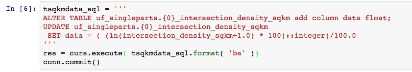
So, recall that a natural log e of 1.0 is 0; a natural log of 116 is slightly over 4.75; a natural log of a number less than 1 is a negative number. To simplify the range for visualization, add a float column called data, set the new data column to the natural log of (intersection_density_sqkm + 1); use a simple multiply-then-divide technique to limit the precision to two digits (screenshot from an IPython Notebook session using psycopg2).

ipython_notebook UPDATE sql

 select quantile(data,ARRAY[0.02,0.25,0.5,0.75,0.92]) from ba_intersection_density_sqkm;
  { 0, 0, 0.52, 1.43, 3.28 }
SELECT
  min(data), 
    quantile(data,ARRAY[0.02,0.25,0.5,0.75,0.92]), 
  max(data) 
FROM ba_intersection_density_sqkm
WHERE data <> 0;

 min  |          quantile          | max  
------+----------------------------+------
 0.21 | {0.21,0.38,0.86,2.17,3.48} | 4.76
(1 row)


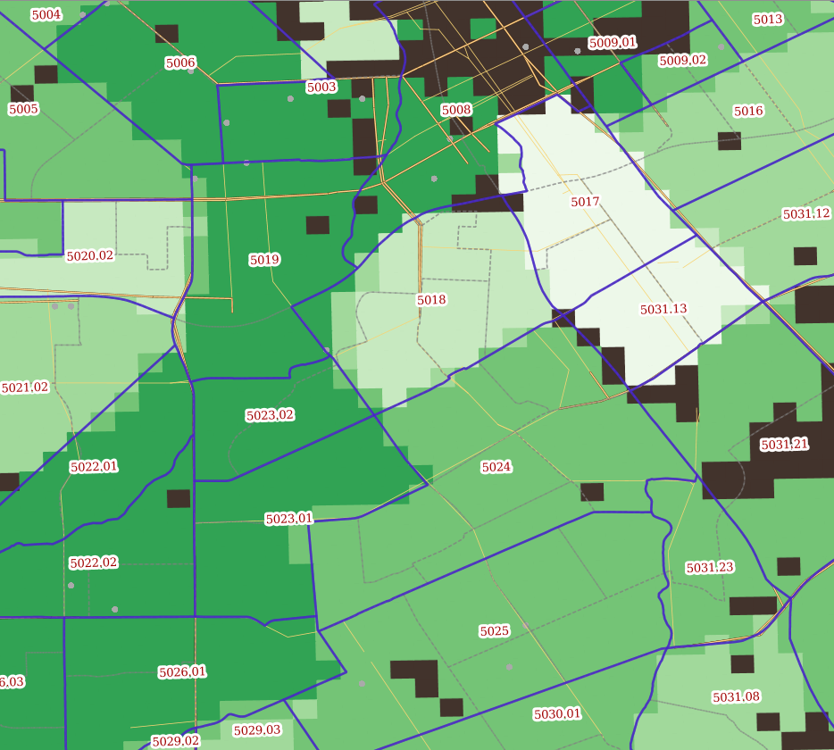
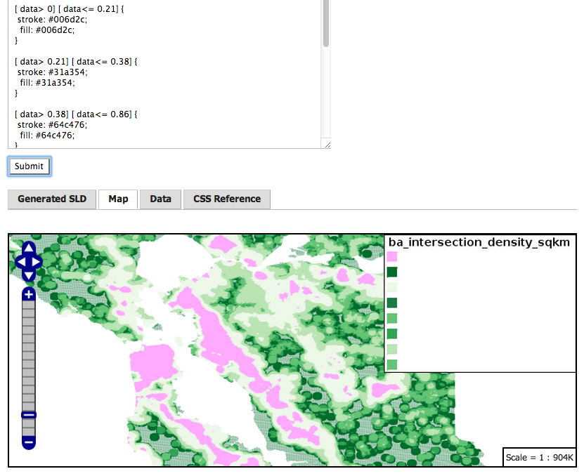
Final Results in GeoServer 2.5 CSS styler:

geoserv_css_style_inters

ps- a full sequential scan on this table takes about four seconds, on a Western Digital Black Label 1TB disk, ext4 filesystem, on Linux.

Debian 7 Repos Added

debian-openlogo-100A small email went by today, bringing big news…
  

From: Jerome Villeneuve Larouche \
To: "ubuntu@lists.osgeo.org" \
Subject: [Ubuntu] DebianGIS Repo

Hello everyone,

This is a small message to tell you that the DebianGIS repo for Debian Wheezy is up and that every package on it is up-to-date! Everything is built against stable so you don't need to add any unstable
repo to use the latest GIS packages. To add it on your machine, edit "/etc/apt/sources.list" and add the line

deb http://debian.mapgears.com/repos/apt/debian/ wheezy main

You should also add the public key here
http://debian.mapgears.com/repos/apt/debian/debgis.gpg.key

Enjoy, as always if you have any questions about the repo, be it this
one or UbuntuGIS, send message on the mailing list!

PS: I'm also currently updating UbuntuGIS to Saucy!

Worldwide Forestry Inventory Published, Nov13

Dozens of major news outlets posted articles yesterday profiling a paper published in the journal ‘Science’ by a team led by Matthew Hansen, a remote sensing scientist at the University of Maryland, along with extensive data.

Hansen_Moore_UMD_forest_delta

Published by Hansen, Potapov, Moore, Hancher et al. * Powered by Google Earth Engine

NCentralCA_Hansen_Moore_etal

NLCD 06 Landcover, San Francisco Bay Area

A colleague pointed out the National Land Cover Database (NLCD) imagery today, which is not new, but it is useful. Here is a simple treatment of the San Francisco Bay Area, with city center markers matching the red urban coloring used in the base map. Click for the larger image, and you can see Lake Tahoe in the East and unmarked is Yosemite National Park almost due south. (’06’ in the blog post title refers to both the publication year of this base map, 2006, and the FIPS code for the State of California)


NLCD_cal_w_cities

California – A Regional Approach

200px-Seal_of_California.svg

A simple spatial classification of geo-data, by federated county; based on the regional planning infrastructure in California.
 

region_defs2

The hilited areas include:


abag_logo


sacog_logo   Sacramento Area Council of Governments


scag_logo
AB32 Scoping Plan Update
Regional Profiles – All


sandag_logo  San Diego Association of Governments


sgc_logo  last but not least, at the State level
 
 
a simple numbering system via postgresql

 region_id |     region_name     
-----------+---------------------
         1 | northern_california
         2 | sierra
         3 | bay_area
         4 | sacramento
         5 | central_valley
         6 | central_coast
         7 | southern_california
         8 | san_diego

California POIs 2013

University_of_California_Seal.svg

I took a short course on the US Census at the University of California, Berkeley D-Lab recently. Of course, the first topic was the shutdown of census.gov. People using the convenient, interactive Census API have been left without access to census data.

Two hours of condensed lecture was just enough time to cover the basics of the breadth of the Census, and the Instructor Dr. Jon Stiles did an expert job.

Following up on some leads from the class, I looked into “points of interest in the 2013 Census data versus OpenStreetMap.” The Census includes a table called pointlm. In the case of California, the file I looked at is called tl_2013_06_pointlm.shp. It is a simple layout, with the state code, an ANSI code, point ID, fullname and something called mtfcc. Rather than dig through 1000 pages of census docs, on a site that is out of service, I found this table , which has an easy to read format and a pointer to the definitions. A quick summary in SQL shows:


US Census

Census 2013 pointlm California
   Definition                           | count
--------------------------------------------------
...
"Hospital/Hospice/Urgent Care Facility" | 292
"School or Academy"                     | 3547
...


OpenStreetMap

OpenStreetMap California latest-snapshot
   Definition                           | count
--------------------------------------------------
...
hospital                                | 829
school                                  | 9201
...

I used a tool called imposm (ignoring the latest-latest new version 3.0 and using the 2.x I was familiar with..) and imported a dump of OpenStreetMap California ‘latest’ to postgresql.

After seeing some of the other counts in the 2013 Census pointlm classes, I quickly became more interested in the OSM dataset for further refinements.

Important Links

ucdata.berkeley.edu
MABLE/Geocorr12
Import “ACS2012 1 Year” to PostgreSQL script
TGRSHP2013_TechDoc.pdf

Distance to Nearest OSM Road

PostgreSQL_logo.3colors.120x120

osm_ca_20=# 
SELECT 
  osm_id, 
  geometry < -> st_geomfromEWKT( 'SRID=900913;POINT(-13145550 4045137)' ) as the_distance
FROM
  osm_new_mainroads 
ORDER BY
  geometry < -> st_geomfromEWKT( 'SRID=900913;POINT(-13145550 4045137)' )  limit 1;


  osm_id  |     the_distance
----------+------------------
 59339590 | 268.205611425265
(1 row)

example_osm_pt_to_road

UPDATE

distance of all museums less than 30km away from a school, by school. Thanks to the geonames project for the locations.

select  
  distinct on (s.name, m.name)
  s.name as school_name, s.admin2, 
  m.name as museum_name, m.admin2, 
  st_distance( s.geom::geography, m.geom::geography )::integer as dist, 
  rank() over ( partition by (s.name, s.admin2)   
    order by st_distance( s.geom::geography, m.geom::geography )) as rank
from   museum m, school s
where 
  s.admin2 = 'Alameda County'  AND 
  m.admin1 = 'California'  AND 
  st_dwithin( m.geom::geography, s.geom::geography, 30000 )
ORDER BY  s.name, m.name, dist;

Five Colors for Stats

PostgreSQL_logo.3colors.120x120

I am building some visualization layers in Geoserver from PostGIS, which requires .sld files (until Geoserver catches up with the CSS styling world – oh wait, look here). It is convenient to show ranges using ColorBrewer2 colors in a set of one plus five.. a color for NoValue, then what I call little0, little1, central value, big1, big0. People often use Standard Deviation for determining the color breaks, but StdDev is based on the average, not the median. In the data I am looking at, it makes a lot more sense to me to take the median value of all values that have a measure, or, a variation on that, all values with a measure and the measure is greater than zero.

In Postgres, I can use an extension called quantile.


a_grid_db=# SELECT
  quantile( pop_assoc_some_coll_pct, ARRAY[ 0.02,0.25,0.75,0.92])
FROM
  ag_edu_assoc_some_coll_pct
WHERE
  pop_assoc_some_coll_pct > 0 and
pop_assoc_some_coll_pct is not null;

quantile
--------------------------------------------
{0.05866,0.14949,0.25696,0.32230}

one_plus_five

In this example, I get approximately: little0 < 0.058; little1 < 0.15; central value > 0.15 and < 0.25; big1 > 0.25 and < 0.32; big0 > 0.32 (filled out completely with boundaries correct). Of course, there are specific reasons to use StdDev and a whole host of statistical techniques, in various situations. This basic technique is good enough for the situation at hand, and so, bears repeating.

PostgreSQL 9.3 plus Hadoop File System

hadoopfdw4logo

It seems that things just got a little bit more interesting with the release of Pg 9.3

Geoserver 2.3 WMS from PostGIS Vectors

geoserver-logo

… it turns out that this technique is important using QGis 1.8 with tiled WMS.


You can set the following options on the wms connection properties:

1) Append this to the wms url "?TRANSPARENT=TRUE" or "&TRANSPARENT=TRUE" if your url already has more parameters

2) Check the option "Ignore GetMap URI reported in capabilities"

This works fine only if your capabilities doc does not point to some other location than the wms url you defined in the connection...

AND ALSO…

   getting fine results with the new QGis 2.0. trying a few experiments now with WMS of PostGIS geometry layers.

AND ALSO…

   Geoserver 2.4 now in place as well.. the block above cost me a lot of hours… grr