Skip to content

Grid 150m classification

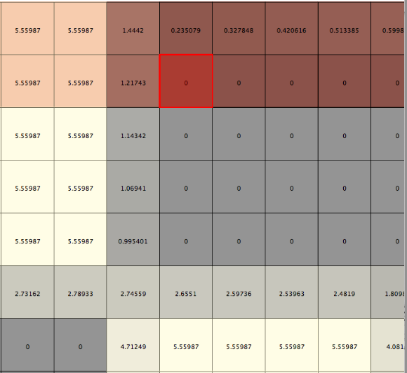
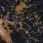
This visualization shows two quantitative dimensions at once, on a 150 meter square grid in a study area in California. The base color is a category of land use, and the gray shading is a percentage of developable acreage. The number on each grid cell, drawn using QGis, is synonymous with the gray shade.

grid150m classifications

Stage of Summarization

Here grid cells are classified into three types by landuse, and county parcels are split along grid cell boundaries, in preparation for computing a result stored into a database table of grid cells as table rows.

Note that roadways, water bodies and some public lands are correctly absent in net calculations, but since the area of a grid cell is a well defined constant, acreage and ratios are trivially computed.

Local Blockgroups 2010

As a way to learn about the geo constructs in the U.S. Census data, I built a few visualizations of the area where I live.


Elementary Constructs 

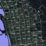
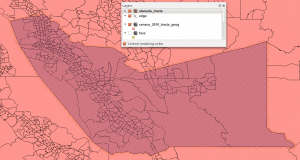
The heavy green lines are census tracts, with their tracts ID shown in large. The pink lines are census block groups. Census blocks are shown, along with the centroid of each. This data comes directly from PostGIS and is styled in QGis


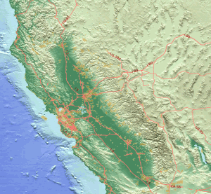
This next image shows the San Francisco Bay Area, Napa Valley to the north, the greater metropolitan area of the state’s capital Sacramento to the southern tip of Lake Tahoe, a portion of the Central Valley down to a corner of Yosemite National Park, then back across Silicon Valley to the Pacific Coast. Each county is divided into census county subdivisions, with its name in yellow. Census place is shown as orange. The heavy pink lines are major highways from OpenStreetMap. Images are served via GeoServer and SLD Styles and again displayed in QGis.

Census data is not the same set as TIGER (Topologically Integrated Geographic Encoding and Referencing) data, but the two are directly matchable via embedded key fields. see the TIGER documentation


Here is the backwards wording from TGRSHP2013_TechDoc, that says that blocks are the indivisible component of all census geometries:

Blocks never cross county or census tract boundaries. They do not cross the boundaries of any entity for which the Census Bureau tabulates data, including American Indian, Alaska Native, and Native Hawaiian areas, congressional districts, county subdivisions, places, state legislative districts, urbanized areas, urban clusters, school districts, voting districts, or ZIP Code Tabulation Areas (ZCTAs) or some special administrative areas such as military installations, and national parks and monuments.

Topology of Hex Cells

A year ago I had modified code from here to make a set of about thirty million hex cells across the continental United States, using the projection from the National Map, EPSG:2163.

Today, topology wizard strk was building a set of hex cells to test conversion to topology in PostGIS 2.0. The question arose, would the hex cells I had built with another method convert cleanly to a topology, and without specifying a tolerance distance?

So I tried converting a subset of the US cells into a topology.
First step, pick a few thousand contiguous hex cells:

-- create one Alameda County multipolygon
DROP TABLE if exists alameda_tracts CASCADE;
CREATE TABLE alameda_tracts as
SELECT 
  1 as ogc_fid, 
  st_union(wkb_geometry) as wkb_geometry
FROM 
  census_2010_tracts
WHERE
  census_2010_tracts.countyfp10 = '001';
ALTER TABLE alameda_tracts add PRIMARY KEY ( ogc_fid );
--
-- transform and compare county to hex cells
DROP TABLE if exists some_hex_cells CASCADE;
CREATE TABLE some_hex_cells as
SELECT 
  distinct on (hex_grid_cells.id, hex_grid_cells.wkb_geometry)
  hex_grid_cells.id, hex_grid_cells.wkb_geometry
  
FROM 
  public.alameda_tracts, 
  public.hex_grid_cells

WHERE 
  ST_Intersects( 
    hex_grid_cells.wkb_geometry,
    ST_Transform(alameda_tracts.wkb_geometry,2163) );
    
--
alter table some_hex_cells add primary key (id);
create index shc_geom_idx on some_hex_cells USING GIST (wkb_geometry);

select count(*) from some_hex_cells;
 count 
-------
  5272
(1 row)

 
In an EXPLAIN ANALYZE of the collection of the hex cells query above, the postgres scheduler showed a linear scan of the table being transformed, which is one record long, and an index scan on the 30 million hex cells – perfect! Next step, create a PostGIS 2.0 topology in EPSG:2163 :

SELECT CreateTopology('hexagon_topo', 2163 );

-- use DropTopology('hexagon_topo') to start over..

 
Now, do the conversion to topology, time it, and validate :

\timing
SELECT TopoGeo_AddPolygon( 'hexagon_topo', h.wkb_geometry )
  FROM some_hex_cells h;

thuban1 Time: 636187 ms
i7-960+ Time: 239265 ms

 select TopologySummary('hexagon_topo');
                        topologysummary                        
---------------------------------------------------------------
 Topology hexagon_topo (2), SRID 2163, precision 0            +
 10608 nodes, 15879 edges, 5272 faces, 0 topogeoms in 0 layers+

It strikes me as odd that the summary would list “0 topogeoms” but if I recall that means that there are no *heirarchical* topologies. Since TopologySummary() returned ok, perhaps my one topology is valid. But, ValidateTopology() returns zero rows ?? I guess there is more to topology to learn, still…

SELECT ValidateTopology('hexagon_topo');
 validatetopology 
------------------
(0 rows)

PS- just noticed this post

PostGIS Geocoder behavior

I became interested in the practical behavior of the

    PostGIS TIGER 2010 Geocoder

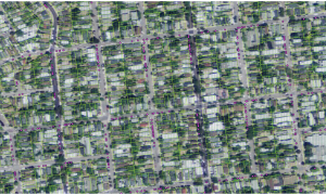
when I started doing statistical profiling of the results of geocoding 100,000 standard addresses in my county and got results that looked like what you see in the image at right. That inquiry morphed into this short paper PDF.

Why statistical profiling? I was experimenting with geocoding a subset of Alameda County parcel records as an example data set after sitting in on most of a graduate Data Mining class at UC Berkeley, Spring 2011. In data mining, any set of attributes that can be reduced to a ‘distance’ measure can be characterized in various ways. With geo-coordinates, distance is obvious, but lexical or numerical relationships can be summarized as ‘distance’ also. Examples of all three occur in geocoding and its data sets.

ST_DWithin on a Grid

As part of a larger inquiry, I wanted to know how ST_DWithin() behaved on a regular grid – that is, what is the relationship of the input radius, and the number of grid cells that could be selected in the result. The manual implies that it is an intersects relationship not a contains relationship, and in this case, the center is not a point but rather an entire grid cell.

Empirically I came up with a formula that does a good enough job of determining a maximum number of grid cells that could be selected (the logic for the inner case of a small radius is rough, but that is almost inconsequential). Here is a SQL query as executed in openJump, and a screenshot:


SELECT  st_asbinary(r.wkb_geometry)
FROM    grid150m_county r
 JOIN    grid150m_county a ON
  ST_DWithin( r.wkg_geometry, a.wkb_geometry, tRadius)
   AND a.ogc_fid = tCellID
GROUP BY
  r.wkb_geometry


A possible Python function to get a maximum count of grid cells:

##-----------------------------------------------------------
import math
def get_gridcell_count( inRadius, inCellSize=150.0 ):

  ## for a given R in meters, get the max number of 150m grid cells 
  ##  that could be included in the results search
  ## Empirically determined to be factorial-like function
  ## adding a new ring at each new grid cell size increment
  ##
  ##  tRadius is in meters
  
  if inRadius < inCellSize:  return 1
  
  tGridCellsSum = 9
  tR = int(math.ceil(tRadius/inCellSize))
  for tInd in xrange(tR):
    tGridCellsSum += int(math.ceil( 2 * (tInd+2) * 3.141592655)) 
  
  return tGridCellsSum

California in Green and Rust

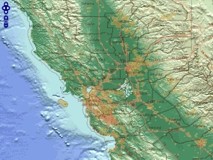
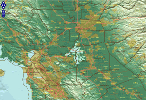
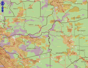
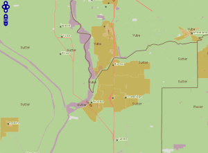
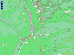
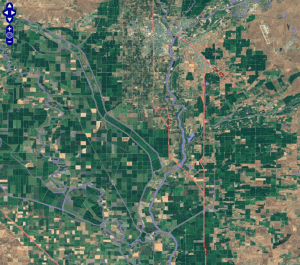
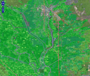
I set out to create a map that showed urban sprawl in the central valley of California.
Geoserver, OpenLayers and PostGIS are the technologies in this demo.
(the linux server itself is being relocated)

gdal_retile retooled

Recently the task of combining and tiling some large GeoTIFFs came up.. so began an investigation of adding threading support to gdal_retile.py

Unfortunately, it is widely known that python is not the best environment for multithreaded work, due to the global interpreter lock (GIL). However, while building threading support for some routine postgis tasks recently, I had quickly found that dispatching a series of computationally intensive PostGIS tasks via psycopg2 in python threading can work quite well. In that case the bulk of the work is done by a large, external engine (PostGIS) and python just acts as a brain to the brawn. I started on this gdal_retile.py experiment with an idea that CPU intensive parts of a gdal_retile.py job, perhaps color-space conversion and JPEG compression, might tip a balance such that the python threading itself was no longer a bottleneck.

I wanted to find a straightforward threading pattern in python that was suitable for breaking up gdal_retile.py’s inner loops.

A Threading Pattern in Python
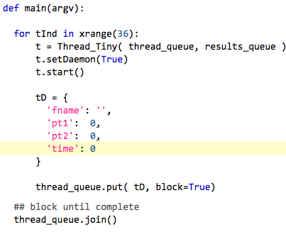
After some experimentation, this program worked well enough.

  • Thread_Tiny is a threading.Thread subclass, whose __init__ function takes two Queue objects as arguments.
  • thread_queue maintains the threads themselves
  • results_queue where each thread pushes its result before being disposed
  • tD a dict containing anything the main program wants to pass to a new Thread
  • put() an args dict into thread_queue. A live thread will pick it up. If all threads are busy working, wait internally until a slot becomes available before adding the queue element
  • app waits for all threads to complete

This construct seemed sufficiently complete to be a template for breaking up a moderately complex utility like gdal_retile.py

Reworking gdal_retile.py
I found that there were really two places that an inner loop repetition was being done. Once where the input was being split into tiles as TileResult_0, and secondly when building a plane of a pyramid TileResult_N. (in gdal_retile.py either operation can be omitted)

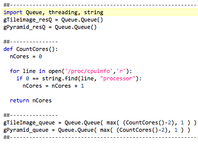
Solution: A utility function Count_Cores() returns the number of cores in the Linux operating environment. Define a thread_queue and result_queue – each instances of Queue.Queue – for each case. A difference is that a thread_queue is created such that there is only one slot per desired active process. This way the thread_queue runs Threads in an orderly way. The number of active Threads is limited to “cores minus two” or one by limiting the number of slots available in a new thread_queue.  Instead of possibly clogging execution with an arbitrarily large set of new Threads to execute at initialization time, only N threads can run at any given time.

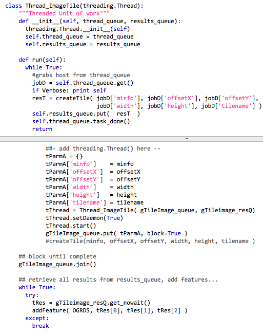
Next, a basic unit of work has to be defined that can be turned over to Threads. In tileImage() there is a call to createTile(), which takes as arguments: a local object called mosaic_info; offsets X,Y; height and width; a tilename; and an object representing an OGR Datasource. That datasource is open and has state, and therefore is not shareable. However I discovered that inside createTile() the only thing the OGR datasource is used for is a single, write-only append of a feature describing the output tile’s BBOX and filename. What if a result_queue replaced the non-shareable datasource passed into createTile() and each thread simply pushes its result into the result_queue ?  When all threads have completed, iterate and retrieve each thread result, adding each to the OGRDS data source as a feature. Here is some code…
A Second Comparison

Fortunately, while discussing this on #gdal Robert Coup (rcoup) happened to be online. In his organization there was another attempt at making gdal_retile.py parallel too, but the results were not satisfying. rcoup tossed the code over, and I ran that as well.

Some Results?

time gdal_retile.py -s_srs EPSG:900913 -co "TILED=YES" -co "COMPRESS=JPEG" -ps 1024 1024 -r "bilinear" -co PHOTOMETRIC=YCBCR -targetDir out_dir_stock Fresno_city_900913.tif

In the end, the version rcoup sent, the threaded version described here, and the stock version, all ran against a 77,000 pixel x 84,000 pixel GeoTIFF (18G, three bands) in about the same 50 minutes each on a local machine (producing a matching 6309 tiles). I suspect that something in the GDAL python interfaces (aside from the GIL) is preventing real parallelism from kicking in, though there are a lot of corners for problems to hide in just this small example.

Long ago, hobu had this to say

Variable Buffers in PostGIS

Some problems in PostGIS are naturally parallelizable. Many problems involving a grid as a base or reference data set fall into this category; when each grid cell is visited and some operation is done there, each grid cell is uniquely referenced in its own set of calculations, and invariant, then it is likely that the problem is naturally parallelizable. If the computation could be done on more than one cell at a time, so much the better.

Search Radii

There are many variations on this problem, and many approaches to solving any given one. Consider the following: a database table representing a regular grid is “loaded” directly with data per cell. The table definition might look like:

create table data_buffers_variable (
    id150 integer PRIMARY KEY, 
    prod_mil_meters double precision,
    wkb_geometry geometry,
    acres_red_total double precision,
    acres_yellow_total double precision,
    qt1 double precision,
    qt2 double precision,
    qt3 double precision
)

 
Each cell will be visited in turn, and reference a number that is a distance prod_mil_meters, which after conversion to units in the current projection, is used as a radius. The calculation is then to collect all cells within the determined radius, and sum three quantities.. qt1_total, qt2_total, qt3_total. Here is a query on a single cell cur_id in a radius of search_radius, and a self-join like so:

SELECT
      b.id150, search_radius, b.wkb_geometry,
  	sum(r.qt1) as qt1_total,
  	sum(r.qt2) as qt2_total,
  	sum(r.qt3) as qt3_total
FROM 
data_buffers_variable b
  INNER JOIN data_buffers_variable r
  ON ST_DWithin(b.wkb_geometry,r.wkb_geometry, search_radius)  AND
  b.id150 = cur_id
  
GROUP BY b.id150, b.wkb_geometry


Many Hands Make Light Work

We might define a function call in PostgreSQL as follows:

CREATE OR REPLACE FUNCTION get_buffered_vals_out(
  in_id_grid int, 
  in_distance float,
  in_geom geometry,
  OUT id_grid int, 
  OUT search_distance float,
  OUT wkb_geometry geometry,
  OUT qt1_total float,
  OUT qt2_total float,
  OUT qt3_total float
  ) 
AS 
$$
  select $1 as id_grid, 
  $2 as search_distance,
  $3 as wkb_geometry, 
  	sum(r.qt1) as qt1_total,
  	sum(r.qt2) as qt2_total,
  	sum(r.qt3) as qt3_total
  FROM data_buffers_variable r WHERE st_dwithin( $3, r.wkb_geometry, $2);
$$ 
COST 10000
language SQL STABLE strict;

 
Now to run this in a parallel fashion. As is detailed in this post, do the following in python: decide on a number of threads to execute, divide the work into buckets with an upper and lower id_grid as bounds, define the basic unit of work as a threading.Thread subclass, and pass a parameter dict into a thread_queue for each thread. Each threaded unit of work will visit each cell within its bounds, call get_buffered_vals_out() and store the results.

note: although it looks more impressive, double precision is in fact a synonym for float in postgres

The syntax for INSERTing the result of a function call like that into another table in one statement can be rather challenging. Here is some useful starter syntax:

select (f).* from (
    select get_buffered_vals_out( ogc_fid, dist, wkb_geometry) as f
    from data_buffers_variable 
    where ogc_fid >= 1656690 and ogc_fid < = 1656690
    offset 0) s;

Why the offset 0 ?!? Its is supposedly a no-op, yet in one test, the runtime is 6x faster with it than without it. More answers yield more questions…

addendum-

whunt	how do you reference a value from the select clause in your where clause?
RhodiumToad	whunt: you don't
whunt	as in: SELECT my_func(bar) as baz from foo where baz is not null;
RhodiumToad	whunt: not allowed per spec, though you can add another nesting level
whunt	i could do it with a with
RhodiumToad	whunt: select * from (select myfunc(...) as baz from ...) s where baz is not null;
RhodiumToad	whunt: note, that'll often call the function twice; to prevent that, add offset 0 just before the )
RhodiumToad	whunt: i.e. select * from (select ... offset 0) s where ...
xocolatl	RhodiumToad: the offset 0 trick is something I think needs improvement we shouldn't have to do that
RhodiumToad	I agree
RhodiumToad	but it's not at all trivial
xocolatl	oh, I don't doubt
whunt	why does the function get run twice?
RhodiumToad	whunt: because the planner will flatten out the subselect in most cases, so it's equivalent to doing
whunt	i imagine the inner query executes the function and creates a new table that the outter query queries
whunt	oh
RhodiumToad	select myfunc(...) from ... where myfunc(...) is not null;
whunt	lol - that's exactly what i wanted to avoid
xocolatl	whunt: then use the offset 0 trick
RhodiumToad	the offset 0 is a general technique to nobble the planner and stop it from flattening subqueries

PostGIS subtraction

Threading in python and calling out to PostGIS in each thread can work well. Here is an example of using python’s Queue and threading.Thread to break up a large spatial workload into pieces. It turns out that many spatial data problems are naturally parallelizable, and this is one of them.

Per the PostGIS manual, subtraction of one geometry from another, ST_Difference( geomA, geomB) might be described as

GeometryA - ST_Intersection(A,B)


A table of geometries can be processed easily if either geomA or geomB is a constant. But what if there are many thousands of geomA, and hundreds of thousands of geomB? Our example is land type classifications (geomA) and California county land parcels (geomB).

Here is a look at a finished result:

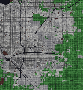
Areas that are colored either green, dark red or gray, are the sum of the area of parcel property in this county, classified into three categories (greenfield, constrained, urban). The remaining yellowish are largely right-of-way (roads, paths, freeways etc). The analysis is done by bringing together two very large input tables – a land classification of the county divided into three classes (14,000 polygons in this example), and the set of parcel properties (~800,000 records).

Start by subtracting all parcels p that touch a given classification polygon l as inner diff

INSERT into landtypes_minus_parcels
SELECT
      l.id_lt,
      l.landtype as landtype_seamless_orig,
      l.other_class,
      CASE when
        st_difference(  l.wkb_geometry,
               st_union(p.wkb_geometry)  )
        is null then l.wkb_geometry
      else
        st_difference(  l.wkb_geometry,
               st_union(p.wkb_geometry)  )
      end
       as tgeom
FROM
   %s l
   inner join
   %s p
   on st_intersects(l.wkb_geometry, p.wkb_geometry)
WHERE l.id_lt = %s
GROUP BY l.id_lt, l.wkb_geometry;

Get a list of primary keys in python from the classification table l

tSQL = '''
select id_lt from %s order by id_lt;
''' % (targ_landtypes)

try:
    gCurs.execute( tSQL )
    gDB.commit()
except Exception, E:
    print str(E)
    raise

idsA  = []
idsTA = gCurs.fetchall()
for tElem in idsTA: idsA.append( tElem[0] )

A psycopg2 query cursor returns an array of tuple – for convenience take the one and only one result per tuple and build a simple list from them. In this analysis, we take the length of the list of primary keys of classification polygons, divide by the desired number of threads, to get a number of classification polygons that will be handled per thread. Since we have an ordered list of primary keys, it is straightforward to pick two keys at a time – upper and lower pkey – and pass them into each thread as dictionary arguments.

tBaseDiv = len( idsA ) / gThreadCount
tBaseOffset = 0
for i in range( gThreadCount ):
    if i == gThreadCount - 1:
       ## last bucket gets any remainder, too
       tEndInd = len( idsA ) - 1
    else:
       tEndInd = tBaseOffset + tBaseDiv - 1

    tD = {
      'start_id': idsA[ tBaseOffset ],
      'end_id': idsA[ tEndInd ]
    }

    tBaseOffset += tBaseDiv
    queue.put( tD )

Next, a unit of work has to be described; a threading.Thread subclass could be defined as follows: upon running, retrieve a parameter Dict from the threads queue, and from it the upper and lower primary key bounds for this thread; for each primary key in this range, execute the inner diff query; when completed, commit() to the database and signal that this thread is complete.

class Thread_ComputeCTWUnit(threading.Thread):
    """Threaded Unit of work"""
    def __init__(self, queue):
      threading.Thread.__init__(self)
      self.queue = queue

    def run(self):
      while True:
        #grabs host from queue
        jobD = self.queue.get()

        tQueuedJobStr = '''
  select id_lt from %s where id_lt >= %s and id_lt < = %s
''' % ( targ_landtypes, jobD['start_id'], jobD['end_id'] )

        #tTmpAnswer = tLocalCurs.fetchone()[0]
        #print 'start_id=',jobD['start_id'],'; end_id=',jobD['end_id'],'; count=',str(tTmpAnswer)

        ##---------------------------
        ## each thread has its own pyscopg2 connection
        try:
          tLocalConn = psycopg2.connect( gDSN )
        except Exception, E:
          print str(E),' start_id=',jobD['start_id']
          self.queue.task_done()
          return

        tLocalCurs = tLocalConn.cursor()
        try:
          tLocalCurs.execute( tQueuedJobStr )
        except Exception, E:
          print str(E)

        tTA_local = tLocalCurs.fetchall()
        for tInd in tTA_local:
            try:
                tLocalCurs.execute( tSQL_primediff % (targ_landtypes,src_parcels,tInd[0]) )
                #tLocalConn.commit()
            except Exception, E:
                print str(E)
                raise

        tLocalConn.commit()
        tLocalConn.close()
        ##---------------------------
        #signals to queue job is done
        self.queue.task_done()
        return

Given 14,000 classified polygons as input, parcel records for a county, running on a 16 core linux machine, and creating 14 threads, each thread will run 1000 queries then commit() back to the database. The runtime in practice is about 15%-30% of the time it would take without threading. One reason for this is that even though each thread has the same number of classification polygons to work on, not all polygon subtractions are created equal, so inevitably some sets of queries take longer than others.